Working with colours in R

When you create a data visualisation using R (or any other software), a set of default colours is used. These aren’t always the most effective, or aesthetically pleasing, set of colours. That means that, at some point, you’ll likely want to use a different set of colours that you have chosen. This blog post will cover how to define those colours in R, where to find examples of colour palettes, and how to make generate your own. It won’t focus too much on how to use these in plots, in base R or {ggplot2}, but there are plenty of good resources out there on this topic, several of which are listed at the end of the post.

To demonstrate some of the palettes that will be used or created in this blog post, we’ll start by creating a function, plot_palette(), that takes a vector of colours and returns a plot showing them.

 1
 2
 3
 4
 5
 6
 7
 8
 9
10
11
12
13
14
15
16

plot_palette <- function(palette) {
 g <- ggplot2::ggplot(
 data = data.frame(
 x = seq_len(length(palette)),
 y = "1",
 fill = palette
 ),
 mapping = ggplot2::aes(
 x = x, y = y, fill = fill
 )
 ) +
 ggplot2::geom_tile() +
 ggplot2::scale_fill_identity() +
 ggplot2::theme_void()
 return(g)
}

Different ways to define colours

There are multiple different ways to define colours in R. We’ll take a look at a few of the most common.

Colour names

Perhaps the easiest way to use colours in R to simply use the name of a colour, written as a character string e.g. "red". You can run colors() to get a list of all the valid colour names. There are currently 657 to choose from – plenty of options other than just "red" or "blue"! Note that all colour names are lowercase, i.e. "red" is a valid colour name but "Red" is not. We can see an example of three of these colours below:

1

plot_palette(c("tomato", "skyblue", "yellow2"))

Hex codes

A very popular way of defining colours (not just in R) is hex codes. Hex codes are of a # followed by a combination of six characters – which can be any of the digits 0 – 9, or any of the letters A – F. This gives 16 options, hence hexadecimal. If you think of hex codes as three pairs of characters then each pair has 16*16 possible combinations which is 256.

In R, hex codes should be written as a character string. If you’re using RStudio, you’ll know it’s a valid hex code because the character string will be highlighted in the colour it defines! You might sometimes see hex codes written with 8 characters rather than 6. The first six characters define the colour as normal, and the last two define the transparency.

1

plot_palette(c("#A053A1", "#DB778F", "#E69F52", "#09A39A", "#5869C7"))

Hex codes can be defined using either upper or lowercase letters (or a mix and match!), and the results are the same, i.e. "#DB778F" and "#db778f" give the same colour. In R, you can also mix and match colour names with hex codes in the one vector e.g. c("black", "#A053A1") will work perfectly fine.

RGB

Another common way of defining a colour is using RGB, which specifies the mixture of Red, Green, and Blue used to create the colour. In R, you can use the rgb() function to define colours in this way. The rgb() function has three arguments that need to be specified, red, green, and blue, which take a vector (of length 1 or longer). For example, the colour defined as rgb(1, 0, 0) is red – 100% red, no green, and no blue. Optionally, you can also set alpha values to change the transparency of the colours.

The arguments can be specified as either a number between 0 and 1, or a number between 0 and some other maxColorValue. The default is between 0 and 1. However, it’s very common to set values between 0 and 255 (giving 256 unique options for each of red, green, and blue, the same as hex codes do). In fact, the rgb() function will actually return a hex code for the colour you’ve defined.

An example of generating three colours using rgb() is shown below:

1
2
3
4
5
6
7

colours <- rgb(
 red = c(32, 243, 176),
 blue = c(52, 62, 200),
 green = c(165, 10, 50),
 maxColorValue = 255
)
plot_palette(colours)

Other definitions

Some other common ways of defining colours are:

• HSV (Hue, Saturation, Value): a colour definition that represents colours based on their hue (type of colour), saturation (intensity or purity of the colour), and value (brightness). In R, you can use the hsv() function e.g. hsv(h = 0.5, s = 0.8, v = 0.9). This function returns a hex code for the colour.
• HCL (Hue, Chroma, Lightness): a colour definition that represents colours based on their hue (type of colour), chroma (intensity or vividness), and lightness (perceived brightness). In R, you can use the hcl() function e.g. hcl(h = 120, c = 50, l = 70). This function also returns a hex code for the colour.

Personally, I use hex codes most often. they give you a wider range of colour options compared to named colours, but are simpler and easier re-use in other software outside of R.

Although the rgb(), hcl(), and hsv() function all return hex codes, and you can use hex codes and colour names in the same vector, there may be times when you need colours in a specific format.

The col2rgb() function (which is part of the {grDevices} package in base R) can convert colours to RGB format.

1

col2rgb(c("red", "#DB778F"))

It returns a matrix with three rows, where each column gives the definition of a different colour:

1
2
3
4

 [,1] [,2]
red 255 219
green 0 119
blue 0 143

The {grDevices} package also has rgb2hsv() function for converting to HSV.
Antti Rask has shared a function for converting from named colours to hex codes. The {plotcolr} package has functions for converting to and from HSL (Hue, Saturation, Lightness which is similar to HSV). The {monochromeR} package also has helper functions for converting between hex codes to RGB and back, with or without transparency. We’ll talk more about these packages later!

Choosing colours

Now that we know how to define different colours, and how to switch between different formats, we need to think about how to decide which colours to actually use.

Colour palettes

There are a few built-in colour palettes that come with the {grDevices} package. For example, the terrain.colors() function:

1

plot_palette(terrain.colors(n = 5))

There are many, many R packages that provide colour palettes. Some are designed to

The
{paletteer} package collects many of these palettes together into a single R package. It also contains functions to use these palettes with {ggplot2} through a series of scale_* functions. You can access the colours using the paletteer_d() or paletteer_c() functions for discrete or continuous palettes, respectively. Simply pass in a character string of the form "{package::palette}".

For example, the
{MetBrewer} package provides a set of colour palettes inspired by paintings in the Metropolitan Museum of Art in New York. The palettes can be accessed directly through the {MetBrewer} package, or through the {paletteer} package:

1
2

library(paletteer)
plot_palette(paletteer_d("MetBrewer::Tara"))

The
Color Palette Finder on the R Graph Gallery offers an easy, interactive way to explore palettes for use in R. You can view different types of palettes (sequential, diverging, or discrete), choose the number of colours, and choose a starting place for the palette e.g. to generate a blue-ish palette.

Accessible choices

Although using colour is not always necessary or the best choice for data visualisations, sometimes it’s unavoidable. When choosing colours for plots, it’s important to think about the accessibility of the colours you are using. There are multiple different types of color vision deficiency (CVD), which affects how people perceive colours. A poor choice of colours may result in your visualisation not being as clear and understandable as you think it is.

There are several packages in R that can be used to assess how colour blind friendly your colour choices are. The cvd_grid() function from the
{colorblindr} package simulates how a plot you’ve created may look to people with colour blindness.

For example, we can test the colours used in a bar chart created with {ggplot2}:

1
2
3
4
5
6
7
8

library(colorblindr)
library(ggplot2)
g <- ggplot() +
 geom_bar(
 data = mpg,
 mapping = aes(y = class, fill = drv)
 )
cvd_grid(g)

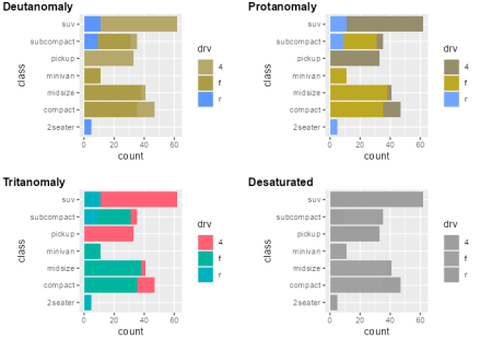
Note that the default colour palette used in {ggplot2} is not very accessible, and the colour for the 4 and f categories are hard to distinguish in the top left. They are also all equally bright, so appear no different when printed in grayscale.

The
{plotcolr} package also shows how colours may look with different types of colour vision deficiency. Rather than passing in an existing plot, you pass in a vector of colours and it shows you how they may look on different types of plots.

Note that here we use names spacing (pre-fixing the function name with the package name and ::) to avoid confusing the plot_palette() function from {plotcolr} with the one we defined at the start of this blog post.

1
2
3
4

plotcolr::plot_palette(
 palette = c("#F75C03", "#D90368", "#04A777", "#820263", "#F4E409"),
 cvd = "all"
)

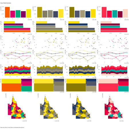
Several other packages exist for similar purposes. The
{colorblindcheck} package can be used to obtain a report about similarity between colours in a vector. The
{cols4all} package has several useful function, including one that launches a GUI to explore different palettes and how accessible they are.

Generating colours

There may be times when you can’t quite find the colour palette you’re looking for and you need to create your own. Note that hand-picking colours is generally not a great idea for plots, since it’s easy to end up with colours that aren’t very accessible. However, for some tasks (such as generative art where sufficient contrast between colours is not the only goal) hand-picked colours may work.

Monochrome palettes

The
{monochromeR} package is designed for creating monochrome colour palettes, based on some colour input. There are options to create a palette that goes lighter than the input colour, darker, or both. There is also an option to blend the input with another colour. For example to blend a palette of 4 colours that goes from orange to pink:

1
2
3
4
5
6
7

library(monochromeR)
generate_palette(
 colour = "#E69F52",
 blend_colour = "#DB778F",
 n_colours = 4,
 view_palette = TRUE
)

The built-in palette plot function from {monochromeR} also prints the hex code in both black and white on each colour, allowing you to see the contrast of text against the background colour.

Blending colours

The colorRampPalette() function from {grDevices} also offers a way to blend together colours. You can pass in a vector of initial colours, and specify how many colours you want out at the end. The function then interpolates the in-between colours, resulting in a colour gradient:

1
2

all_colours <- colorRampPalette(c("tomato", "skyblue", "yellow2"))(100)
plot_palette(all_colours)

Generating 100 of colours on a gradient may not be that useful in itself, but you can then take a random sample of these colours. This often results in a palette that appears harmonised because they are all generated from the same set of blended colours:

1
2
3

set.seed(123)
choose_colours <- sample(all_colours, n = 5)
plot_palette(choose_colours)

Random hex codes

Both of the approaches mentioned so far require some initial input colour(s). So how do you decide on that? One approach is to start with a colour at random. The
coolors.co website is a great way to generate a random set of colours. You can then use one or more of these as your initial starting colour(s).

However, we can also generate random colours in R. Let’s create a random_hex() function that generates as many random hex codes as we want (given by the argument n).

We start by constructing a vector containing the digits 0-9 and the letters A-F, sample (with replacement) six of these values at random, and squash them into a single character, pre-fixed by #. We then call that function n times, and return a character vector of length n.

1
2
3
4
5
6
7
8
9

random_hex <- function(n) {
 generate_hex <- function() {
 choices <- sample(c(as.character(0:9), LETTERS[1:6]), size = 6, replace = TRUE)
 output <- paste0("#", stringr::str_flatten(choices))
 return(output)
 }
 hex <- replicate(n = n, generate_hex(), simplify = TRUE)
 return(hex)
}

We can then generate colours using our random_hex() function, remembering to set a random seed so we can re-create the palette again:

1
2

set.seed(123)
plot_palette(random_hex(6))

Colours from images

Another option is to use an image as your starting point. This might be a company logo, or an image related to the data you are plotting, for example. There are several online tools for generating palettes from images but, again, we can do this directly in R! The
{eyedroppeR} package is designed for picking colours from images. The eyedropper() function allows you to interactively click on an image and then returns the hex code of the pixel you clicked on. The extract_pal() function goes one step further, and extracts your chosen number of colours from the image for you. You can pass in either a local image or a URL to one online. Here, we’ll use the image of a river from a previous blog post on
creating typewriter-styled images in R.

We could use our own palette plotting function, but the {eyedroppeR} package has it’s own swatch() function which is used automatically:

1
2
3
4
5

library(eyedroppeR)
extract_pal(
 n = 4,
 img_path = "https://nrennie.rbind.io/blog/creating-typewriter-images-r/image.jpg"
)

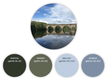
Further reading

If you’d like to continue reading about working with colours in R, these are some good places to start:

• Cara Thompson has many useful resources about choosing colours in R, including the
  resources from her NHS-R conference talk on creating and applying bespoke colour schemes.

• I previously wrote a
  blog post for Jumping Rivers about how to create your own custom colour palette functions if you want to make it easier to use your chosen colours in {ggplot2}.

• This one isn’t R specific but it’s insanely useful! Lisa Muth’s
  Datawrapper blog post contains lots of design tips for creating your own colour palette.

Related