[This article was first published on r.iresmi.net, and kindly contributed to R-bloggers]. (You can report issue about the content on this page here)
Want to share your content on R-bloggers? click here if you have a blog, or here if you don’t.
Day 5 of 30DayMapChallenge: « A Journey » (previously).
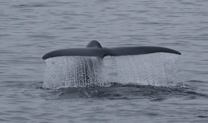
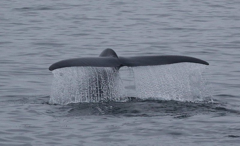
Thirteen Blue whales (Balaenoptera musculus) were satellite tagged in 2015 in Australia (Mӧller et al. 2020). We’ll follow their summer in the Great Southern Australian Coastal Upwelling System (GSACUS).
Data is available from the Australian Antarctic Data Centre (Andrews-Goff et al. 2020), directly as a R RDS file.
library(dplyr)
library(readr)
library(sf)
library(leaflet)

unzip("AAS_4101_pygmy_blue_whale_SSSM.zip",
      files = "bw_3h_ssm.RDS")
bm <- read_rds("bw_3h_ssm.RDS")
# str(bm)

journeys <- bm$summary |>
  st_as_sf(coords = c("lon", "lat"), crs = "EPSG:4326") |>
  group_by(id) |>
  arrange(date) |>
  summarise(do_union = FALSE) %>%
  st_cast("LINESTRING") |>
  group_by(indiv = as.factor(parse_number(as.character(id)))) |>
  summarise()
After joining GPS points as lines and lines from the same whale as multilines, we can use {leaflet} for an interactive map.
pal <- colorFactor("viridis", sort(unique(journeys$indiv)))

journeys |>
  leaflet() |>
  addTiles() |>
  addPolylines(color = ~ pal(indiv),
               popup = ~ indiv) |>
  addLegend(pal = pal,
            values = sort(unique(journeys$indiv)))


