Time Series Machine Learning: Shanghai Composite

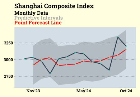
Shanghai Composite does not seem to be at an ideal point for entry.

Source code:

library(tidyverse)
library(tidyquant)
library(timetk)
library(tidymodels)
library(modeltime)
library(workflowsets)

#Shanghai Composite Index (000001.SS)
df_shanghai <- 
  tq_get("000001.SS", from = "2015-09-01") %>% 
  tq_transmute(select = close,
               mutate_fun = to.monthly,
               col_rename = "sse") %>% 
  mutate(date = as.Date(date)) 

#Splitting
split <- 
  df_shanghai %>% 
  time_series_split(assess = "1 year", 
                    cumulative = TRUE)

df_train <- training(split)
df_test <- testing(split)

#Time series cross validation for tuning
df_folds <- time_series_cv(df_train,
                           initial = 77, 
                           assess = 12)


#Preprocessing 
rec <- 
  recipe(sse ~ date, data = df_train) %>% 
  step_mutate(date_num = as.numeric(date)) %>% 
  step_date(date, features = "month") %>% 
  step_dummy(date_month, one_hot = TRUE) %>% 
  step_normalize(all_numeric_predictors())


rec %>% 
  prep() %>% 
  bake(new_data = NULL) %>% view()


#Model
mod <- 
  arima_boost(
    min_n = tune(),
    learn_rate = tune(),
    trees = tune()
  ) %>%
  set_engine(engine = "auto_arima_xgboost")

#Workflow set
wflow_mod <- 
  workflow_set(
    preproc = list(rec = rec),
    models = list(mod = mod)
  ) 


#Tuning and evaluating the model on all the samples
grid_ctrl <-
  control_grid(
    save_pred = TRUE,
    parallel_over = "everything",
    save_workflow = TRUE
  )

grid_results <-
  wflow_mod %>%
  workflow_map(
    seed = 98765,
    resamples = df_folds,
    grid = 10,
    control = grid_ctrl
  )


#Accuracy of the grid results
grid_results %>% 
  rank_results(select_best = TRUE, 
               rank_metric = "rmse") %>%
  select(Models = wflow_id, .metric, mean)


#Finalizing the model with the best parameters
best_param <- 
  grid_results %>%
  extract_workflow_set_result("rec_mod") %>% 
  select_best(metric = "rmse")


wflw_fit <- 
  grid_results %>% 
  extract_workflow("rec_mod") %>% 
  finalize_workflow(best_param) %>% 
  fit(df_train)


#Calibrate the model to the testing set
calibration_boost <- 
  wflw_fit %>%
  modeltime_calibrate(new_data = df_test)

#Accuracy of the finalized model
calibration_boost %>%
  modeltime_accuracy(metric_set = metric_set(mape, smape))



#Predictive intervals
calibration_boost %>%
  modeltime_forecast(actual_data = df_merged %>% 
                       filter(date >= last(date) - months(12)),
                     new_data = df_test) %>%
  plot_modeltime_forecast(.interactive = FALSE,
                          .legend_show = FALSE,
                          .line_size = 1.5,
                          .color_lab = "",
                          .title = "Shanghai Composite Index") +
  geom_point(aes(color = .key)) +
  labs(subtitle = "Monthly Data
Predictive Intervals
Point Forecast Line") + 
  scale_x_date(breaks = c(make_date(2023,11,1), 
                          make_date(2024,5,1),
                          make_date(2024,10,1)),
               labels = scales::label_date(format = "%b'%y"),
               expand = expansion(mult = c(.1, .1))) +
  ggthemes::theme_wsj(
    base_family = "Roboto Slab",
    title_family = "Roboto Slab",
    color = "blue",
    base_size = 12) +
  theme(legend.position = "none",
        plot.background = element_rect(fill = "lightyellow", color = "lightyellow"),
        plot.title = element_text(size = 24),
        axis.text = element_text(size = 16),
        plot.subtitle = ggtext::element_markdown(size = 20, face = "bold"))

Related