Want to share your content on R-bloggers? click here if you have a blog, or here if you don’t.
R functions for every data engineer using Tidyverse
Tidyverse has long been an amazing collection of R packages, primarily for data engineering and data science. Common among these packages is the same language grammar, great design and structure, making data science easier.
Motivation
Data engineering is important step that helps improve data usability, data exploration and data science. Preparing the data needs therefore needs to be done in a manner, that is easy to read, repeat and exchange between others engineers.
Tidyverse has a lot of data engineering functions, chaining different functions for getting most of your data. All six examples will show combinations of functions chained together for great result set.
The following R code is based on open datasets called mtcars, that is available with base R engine.
1. Applying transformations or models to grouped data
Combining aggregated data to grouped data or original dataset is frequently used data manipulation technique for extracting and calculating ratios, percentages, cumulatives or growth calculations (e.g.: YoY).
mtcars %>%
  group_by(cyl) %>%
  nest() %>%
  mutate(
    summary_stats_for_cyl = map(data, ~ summarise(.x,
                                          mean_mpg_per_cyl_group = mean(mpg),
                                          sd_mpg_per_cyl_group = sd(mpg)
                                          )
                        )
  ) %>%
 unnest(cols = c(data, summary_stats_for_cyl))
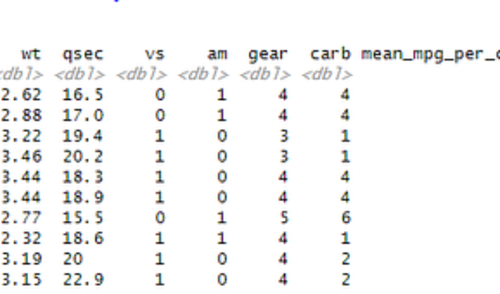
With nest() function and map() over summarise() we can get the for each group of cylinder cars a grouped values for mean and standard deviation.


2. Pivot wide data and apply transformations to all variables
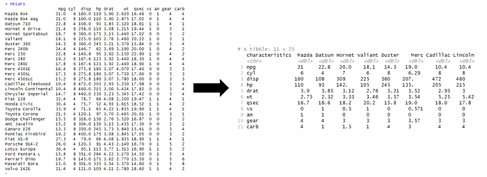
Pivoting data is powerful function for calculating aggregations, and in this example we are pivoting longer and wider on car brand, where all the values have applied aggregation function of mean().
In addition, we also add the total average and total standard deviation of all car brands for each of the car characteristic.
Tidyverse code is simple to understand and easy to read.
mtcars %>%
   mutate(brand = word(rownames(.), 1)) %>%
   pivot_longer(cols = !brand, names_to = "characteristics", values_to = "value") %>%
   pivot_wider (names_from = "brand", values_from = "value", values_fn = ~ mean(.x, na.rm = TRUE)) %>%
   mutate(
    mean_charac = rowMeans(across(where(is.numeric)), na.rm = TRUE),
    sd_charac = apply(across(where(is.numeric)), 1, sd, na.rm = TRUE)
  )
And the transformation is informative and useful for e.g.: comparison between the brands.


3. Pivoting data for purposes of data cleaning
Usual data engineering case is to fill-in the missing values or replace them with other values. In this case, we are transforming wide data to long format, fill missing values, and pivot back to the original wide format. Reason for pivoting data is to impute the missing values based on the median value. It could also be the last non-missing value in a long dataset, or it can also be ordered by time, size or running ID and populated backward or forward.
df_ts <- tibble(
  id = 1:4,
  year_2021 = c(100, 200, NA, 400),
  year_2022 = c(150, NA, 300, 450),
  year_2024 = c(240, NA, NA, NA)
)

df_ts %>%
  pivot_longer(cols = starts_with("year"), names_to = "year", values_to = "value") %>%
  mutate(value = replace_na(value, median(value, na.rm = TRUE))) %>%
  pivot_wider(names_from = year, values_from = value)
In this case, the median value for all years (year_2021,year_2022, year_2024) is calculated (value = 240) and replaced with all the missing value indicators.


4. Time-series interpolation and creating rolling aggregates
Working with time-series dataset often requires to clean the data by replacing outliers or missing values. In addition, normally we also want to create additional features from original data points.
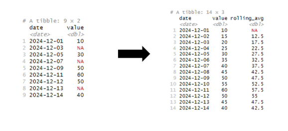
In the following example, we will add the missing dates to the time series (as we are using daily data) by using complete() function. In the next step, we will use interpolation on missing intervals and overwrite the values in value column. And finally, we will use rollapply() function to calculate rolling average over the window of two days (hence width =2).
library(zoo)

df <- tibble(
  date = as.Date("2024-12-01") + c(0, 2, 4, 6, 8, 10, 11, 12, 13),
  value = c(10, NA, 30, NA, 50, 60, 50, NA, 40)
 )

df %>%
  complete(date = seq.Date(min(date), max(date), by = "day")) %>%
  mutate(value = zoo::na.approx(value, na.rm = FALSE)) %>%
  mutate(rolling_avg = rollapply(value, width = 2, align = "right", fill = NA, FUN = mean))
With simple combination of rollapply() and na.approx() functions (both from library zoo), we can quickly do a lot of steps in tidyverse manner.


5. Cross-tabulations with margins and total percentages
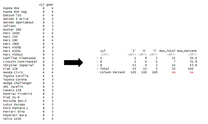
Combining the power of bind_rows() function, complete(), pivot functions and across() we can create a cross-tabulation matrix between two variables in mtcars; cyl and gear.
cross_tab <- mtcars %>%
   count(cyl, gear) %>%
   complete(cyl = unique(mtcars$cyl), gear = unique(mtcars$gear), fill = list(n = 0)) %>%
   pivot_wider(names_from = gear, values_from = n, values_fill = list(n = 0)) %>%
   mutate(
     cyl = as.character(cyl),
     Row_Total = rowSums(select(., -c(cyl)))
   ) %>%
   mutate(
     Row_Percent = round(Row_Total / sum(Row_Total) * 100, 2)
   ) %>%
   bind_rows(
     summarise(
       .,
       cyl = "Total",
       across(-c(cyl), sum, na.rm = TRUE),
       Row_Percent = 100
     )
   )

column_percent <- cross_tab %>%
 filter(cyl == "Total") %>%
 mutate(
   cyl = "Column Percent",
   across(-c(cyl, Row_Total, Row_Percent), ~ round(.x / sum(.x) * 100, 2)),
   Row_Total = NA,
   Row_Percent = NA
 )

final_table <- bind_rows(cross_tab, column_percent)
print(final_table)
This script calculates margin statistics and percentages over the values for each group in given column with respect to each row.


6. Applying function map from purrr
Package purrr (as part of tidyverse) is a powerful set of functions for functional programming for working with functions and vectors. Functions map() is an easy and a great way to replace for loops in your code. This pattern of looping over a vector, and doing an operation to each of the elements and storing the results is the main advantage of purrr package over R-base functions.
In the snippet below, we create a function called apply_funs that accepts an argument for data frame (that is broken down to individual vector) and applies family of statistical functions, like median, mean, standard deviations and others.
In both examples, we are using map function and for looping over values of a vector or looping over a list of vectors (in this case a data frame).
# for vector
apply_funs_vec <- function(x, ...) {
  purrr::map_dbl(list(...), ~ .x(x))
}

apply_funs_vec(mtcars$cyl, mean, median, sd, min, max)

#for dataframe (or vector)
apply_funs <- function(x, ...) {
  funs <- list(...)
  fun_names <- as.character(substitute(list(...))[-1])

  if (is.data.frame(x)) {
    x <- dplyr::select_if(x, is.numeric)
    results <- purrr::map_dfc(x, function(column) {
      purrr::map_dbl(funs, ~ .x(column))
    })
    results <- as.data.frame(results)
    rownames(results) <- fun_names
    return(results)

  } else if (is.numeric(x)) {
    results <- purrr::set_names(purrr::map_dbl(funs, ~ .x(x)), fun_names)
    return(results)
  } else print("Need numeric input")
}

apply_funs(mtcars, mean, median, sd, min, max)
apply_funs(mtcars$cyl, mean, median, sd, min, max)


## or with map_df
mtcars_res <- mtcars %>%
  map_df( ~ list(
                mean = mean(.),
                median = median(.),
                sd = sd(.),
                min = min(.),
                max = max(.)
    )
)

mtcars_res <- t(mtcars_res)
colnames(mtcars_res) <- names(mtcars)
mtcars_res
And the result of map() function is an overall descriptive statistics for all numeric variables.


Conclusion
This shortlist of Tidyverse combinations is not only a helpful list, but also a display of powerful toolkit of functionalities for everyday work for data scientists and data related roles. With the language of Tidyverse, your code will also be simpler and easier to read, thus making it more manageable.
As always, code is available at my Github repository.
Happy R-Coding and happy new year 2025!
Article was first published on Medium (31.12.2024)
Related


