I have been thinking in my spare time a bit about synthetic control methods as an approach to evaluation, and am working on a blog post. But a side issue that popped up was sufficiently interesting to treat separately.
Technically, it is a question of fitting a regression where the coefficients are constrained to be non-negative and add up to one; in other words, the coefficients are a simplex. The reason this comes up is in that in synthetic control methods, such a regression is used to determine the weights to use in constructing a weighted average of multiple units (countries, firms, people) that is as comparable as possible to the unit that received the intervention being evaluated.
The argument for the weights adding up to one is to avoid extrapolating from the range of the real data. I don’t find this a convincing argument, but I’ll leave that for a later post if I get round to it. For now, I’m interested in the technical question of how to get such a set of non-zero weights adding up to one; or abstracting it away from the application, how to fit a regression where the coefficients are constrained to be a simplex.
Naturally, there are multiple ways you might do this. There was a good question and answer on this on Cross-Validated way back in 2012. Two of the four methods I’m going to go through below come pretty much straight from answers or comments there. The other two are my own invention (I’m not claiming to be the first, just that I haven’t seen others doing it this way).
First, let’s get started by simulating some data. I’m going to make a matrix called X with five columns, all from different distributions. Then I create a vector of true coefficients that will relate the y I’m about to make to that X. To make the exercise interesting and life-like, the true coefficients are going to involve a negative number, and aren’t going to add to exactly 1. One of them is going to be zero.
library(glmnet)
library(MASS)   # for eqscplot
library(pracma) # for lsqlincon
library(rstan)
options(mc.cores = min(8, parallel::detectCores())
par(bty = "l", family = "Roboto")

n <- 1000
X <- cbind(
  x1 = rnorm(n , 10, 2),
  x2 = rnorm(n, 7, 1),
  x3 = rnorm(n, 15, 3),
  x4 = runif(n, 5, 20),
  x5 = rnorm(n, 8, 1.5)
)
# note true data generating process coefficients add up
# to more than 1 and have a negative, to make it interesting
true_coefs <- c(0.2, 0.6, -0.1, 0, 0.4)

y <- X %*% true_coefs + rnorm(n, 0, 2)
Now, I’m going to fit various regressions (with no intercept) to this data and extract the coefficients and compare them to the true data generating process. First let’s start with ordinary least squares with no constraints
#-------------method 1 - unconstrained regression------
# This is the best way to recover the true DGP
mod1 <- lm(y ~ X - 1)
coefs1 <- coef(mod1)

# plotting function we will use for each model
f <- function(newx, main = ""){
  eqscplot(true_coefs, newx, bty = "l",
           xlab = "Coefficients from original data generating process",
           ylab = "Coefficients from model",
           main = main)
  abline(0, 1, col = "grey")
  }
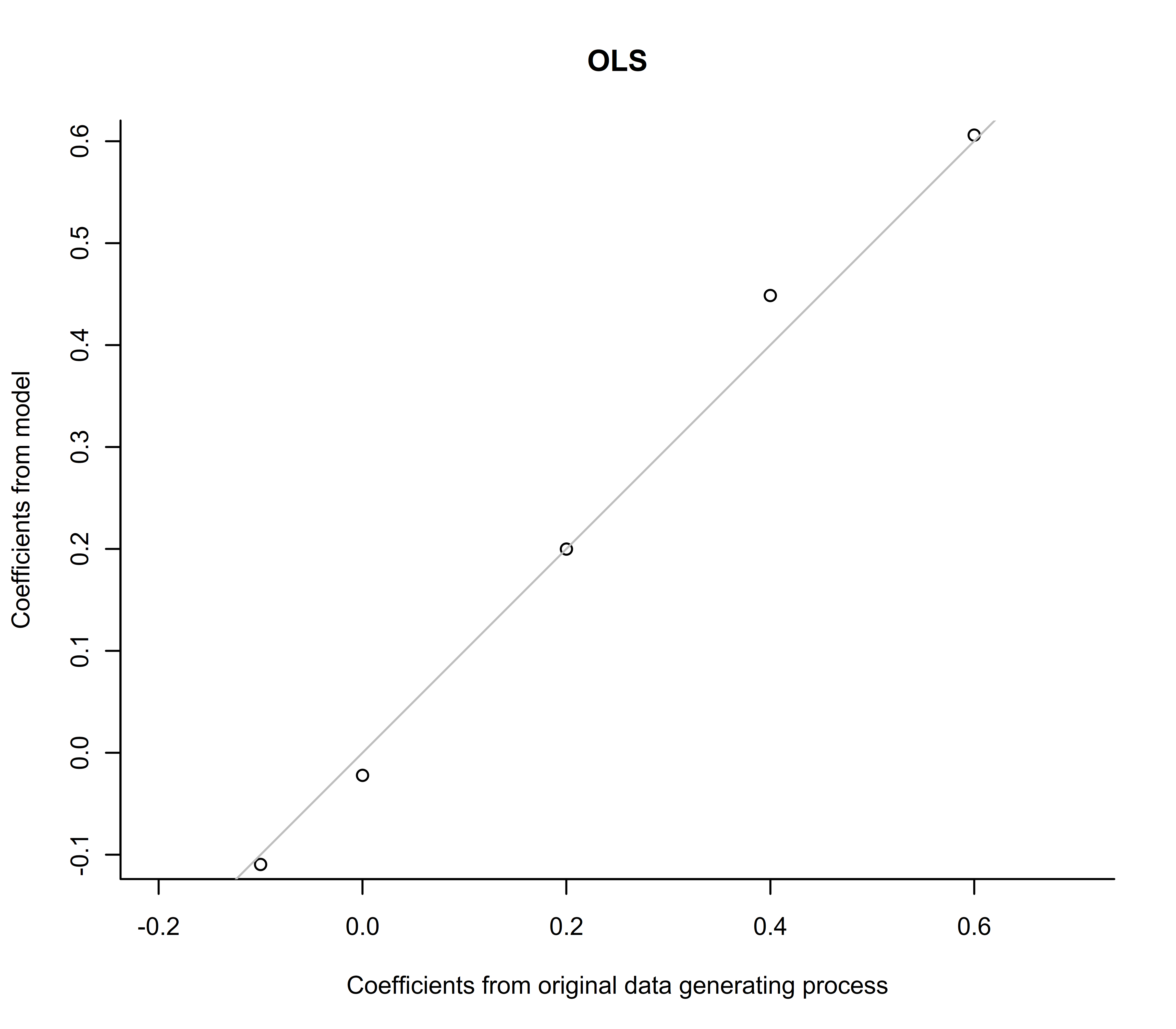
f(coefs1, "OLS")
This approach is very good at getting close to the true data generating process, as we’d expect. But of course, like the true process, it has a negative coefficient for x3, and it sums to more than 1:
> round(coefs1, 2)
  Xx1   Xx2   Xx3   Xx4   Xx5
 0.20  0.61 -0.11 -0.02  0.45
> sum(coefs1)
[1] 1.122484
This is the plot we get, comparing the model’s coefficients to those from the real data generating process:
OK, all very good but it makes no effort (other than just hoping it works out) to constrain the coefficients to add up to one. So here’s my first real attempt at that, which is based on a suggestion that whuber made in the comments on the Cross-Validated post. He points out with some basic algebra that if you subtract one of the X columns from the others and from y, and then fit a regression with OLS to that transformed data, you get the correct coefficients on all the columns of X that you left in, and can calculate the remaining one by just subtracting them all from 1.
#-----------method 2 - transform-----------
# This way will get you coefficients that add up to 1,
# but might not be in (0, 1). This is suggested by whuber in
# his comment on Elvis' solution at:
# https://stats.stackexchange.com/questions/21565/how-do-i-fit-a-constrained-regression-in-r-so-that-coefficients-total-1
X2 <- X[, 1:4] - X[, 5]
y2 <- y - X[, 5]

mod2 <- lm(y2 ~ X2 - 1)
coefs2 <- c(coef(mod2), 1 - sum(coef(mod2)))
f(coefs2, "Transformation") # draw plot
This time the coefficients add up exactly to one as required, but unfortunately there is still a negative in there
> round(coefs2, 2)
 X2x1  X2x2  X2x3  X2x4
 0.24  0.40 -0.04  0.00  0.40
> sum(coefs2)
[1] 1
This isn’t news – it was identified as a problem in the discussion on Cross-Validated, but with the simulated data used there it didn’t manifest. In fact, this is one reason why my simulated data is a bit dirtier, with original coefficients that don’t add to one and which have a genuine negative value among them.
So much for model 2.
Model 3 is one I invented myself and makes use of the fact that glmnet lets you not only regularise your coefficients (squash them towards zero, to help handle multicollinearity, overfitting, and related issues) it lets you specify upper and lower bounds for coefficients. So we could get our first fully compliant set of regression coefficients (non-negative, adding to one) by using the data transformation approach in model2 but fitting the model with glmnet instead. Like this:
#----------method 3 - transform, regularise and constrain-----------
# This method is guaranteed to get you coefficients that add up to 1,
# and they will also be in the (0, 1) range, plus they will be regularised

# alpha = 0 is ridge regression, but could use 1 for lasso (or anything in between)
mod3 <- cv.glmnet(X2, y2, intercept = FALSE, alpha = 0,
                  lower.limits = 0, upper.limits = 1)

# Coefficients from glmnet include the intercept even though we forced it to be zero
# which is why we need the [-1] in the below
coefs3 <- c(as.vector(coef(mod3)[-1]), 1 - sum(coef(mod3)))
f(coefs3, "Transform and ridge") # draw plot
The results are all non-negative, and add correctly to one:
> round(coefs3, 2)
[1] 0.11 0.24 0.00 0.00 0.64
> sum(coefs3)
[1] 1
They do differ markedly from the true coefficients:
We’ll come back to that.
Next is what we might call the “proper” solution, which is to treat the problem as the classic case for quadratic programming that it is. Quadratic programming was developed exactly to deal with this situation – optimise a multivariate quadratic function (like, least squares in a regression) subject to linear constraints (like, coefficients must be non-negative and add up to one). Hans Borchers’ R package (“Practical Numerical Math Functions”) has an easy to understand interface to do this without having to invert your own matrices, so the only thing you need to do is to express the constraints in the right way. Here’s how we do this with our problem:
#---------------method 4 - quadratic programming-----------------
# This is based on dariober's solution, which itself is Elvis' solution
# but using the easier API from pracma::lsqlincon
# lsqlincon "solves linearly constrained linear least-squares problems"

# Equality constraint: We want the sum of the coefficients to be 1.
# I.e. Aeq x == beq
Aeq <- matrix(rep(1, ncol(X)), nrow= 1)
beq <- c(1)

# Lower and upper bounds of the parameters, i.e [0, 1]
lb <- rep(0, ncol(X))
ub <- rep(1, ncol(X))

# And solve:
coefs4 <- lsqlincon(X, y, Aeq= Aeq, beq= beq, lb= lb, ub= ub)

f(coefs4, "Quadratic programming")
Just like the previous method, our result is all non-negative and sums to zero:
> round(coefs4, 2)
[1] 0.17 0.44 0.00 0.00 0.38
> sum(coefs4)
[1] 1
This time the coefficients look a bit closer to the original ones:
Finally, I the other method I invented was to go all-in Bayesian and simply specify in Stan that the coefficients have to be a simplex and that they have a Dirichlet distribution. This actually seems the most intuitive solution to me – what better way is there of making something a simplex than by just deeming it to have a Dirichlet distribution?
So I wrote this program in Stan:
// Stan program for a regression where the coefficients are a simplex
// Probable use case is when y is some kind of weighted average of the X
// and you want to guarantee the weights add up to 1 (note - note sure I think
// this is a good idea but it is out there)
//
// Peter Ellis November 2024

data {
  int n;   // number of data items must match number rows of X
  int k;   // number of predictors must match number columns of X
  matrix[n, k] X;   // predictor matrix. Might include intercept (column of 1s)
  vector[n] y;      // outcome vector
}
parameters {
  simplex[k] b;       // coefficients for predictors
  real sigma;  // error scale
  real alpha; // parameter for dirichlet distribution
}
model {
  alpha ~ beta(2, 2);
  b ~ dirichlet(rep_vector(alpha, k));
  y ~ normal(X * b, sigma);  // likelihood
}
… and called it from R with this:
#----------------method 5 - Bayesian model with a Dirichlet distribution------
stan_data <- list(
  n = nrow(X),
  k = ncol(X),
  X = X,
  y = as.vector(y)
)

mod5 <- stan("0281b-dirichlet-coefs.stan", data = stan_data)

coefs5 <- apply(extract(mod5, "b")$b,2, mean)
This is now the third method for which our result is correctly all non-negative and sums to zero:
> round(coefs5, 2)
[1] 0.17 0.45 0.00 0.00 0.38
> sum(coefs5)
[1] 1
… and this is what it looks like, basically very similar to the quadratic programming solution:
OK, which method is best? We need some sort of benchmark to test them against, better than the original coefficients from the data generating process in complying with the fundamental restrictions. Given the ultimate purpose is to construct a weighted average, we want something that has similar proportions to the original coefficients. So, just wanting to be pragmatic about this, I created a “normalised” set of coefficients by removing the negative one and scaling the remainder to add up to one.
This lets us define a success criteria – the winning method is the one that meets the constraints (ruling out models 1 and 2) and most closely matches those proportions. Here’s a nice pairs plot comparing everything at a glance:
What we see is that models 4 and 5 are clear, effectively equal, winners. Not only are they nearly identical, they also match the normalised true coefficients (correlations of 0.98 or above). Sadly, the glmnet method doesn’t perform very well at recovering the original proportions. Perhaps it would have done better if I’d let the columns of X be correlated with eachother rather than independent (dealing with multi-collinearity being elastic net regression’s home turf). Perhaps also it would get closer to the quadratic programming solution if I forced the amount of regularisation down to nearly zero. But with two good solutions already I’m not inclined right now to experiment further on that.
The quadratic programming approach was easier to write and debug and quicker to run than the explicit modelling of the Dirichlet distribution in Stan, so pragmatically it becomes the winner; with the sole caveat being that question mark in the last paragraph about what happens if the columns of X are multi-collinear.
Oh, let’s finish with the code to draw that pairs plot. For one reason or another, I used good old base R pairs() to do this, rather the GGally package I more normally use for scatterplot matrices. I like the easy control pairs() gives you over the upper and lower triangles of the scatterplot matrix, by just defining your own function on the fly. So for the old-timers, here’s that base R code:
#---------------comparisons------------
norm_coefs <- pmax(0, true_coefs) # remove negative values
norm_coefs <- norm_coefs / sum(norm_coefs) # force to ad dup to one

pairs(cbind('Actual data\ngenerating process' = true_coefs,
            'Normalised to\nadd to one and > 0' = norm_coefs,
            "Ordinary least squares,\nwon't add to 1, not\nconstrained to (0,1)" = coefs1,
            'Transform and OLS, add to 1\nbut can be negative' = coefs2,
            'Transform and ridge regression,\nconstrain to within (0,1)' = coefs3,
            'Quadratic programming' = coefs4,
            'Dirichlet & Stan' = coefs5),
      lower.panel = function(x, y){
        abline(0, 1, col = "grey")
        points(x, y, pch = 19)
      },
      upper.panel = function(x, y){
        text(mean(range(x)), mean(range(y)), round(cor(x, y), 2),
             col = "steelblue", font = 2)
        },
       main = "Comparison of different methods for creating a weighted average with weights adding up to one")
Related


