Hexagonal grid?
We will do statistical binning on a hexagonal grid, but not just any grid. Geodesic Discrete Global Grid Systems (Kimerling et al. 1999; Sahr, White, and Kimerling 2003) allow to use hierarchical equal-area hexagon1 grids.
The {dggridR} package (Barnes 2017) will help us to generate these grids on France.
library(dggridR)
library(dplyr)
library(purrr)
library(sf)
library(units)
library(glue)
library(tibble)
library(ggplot2)
library(ggspatial)
library(rnaturalearth)
# devtools::install_github("ropensci/rnaturalearthhires")
First we are going to build these Discrete global grids for metropolitan France with cell size of 1, 5, 10, 20 and 100 km. We need a spatial footprint.
# get it from
# https://static.data.gouv.fr/resources/admin-express-cog-simplifiee-2024-metropole-drom-saint-martin-saint-barthelemy/20240930-094021/adminexpress-cog-simpl-000-2024.gpkg
fx <- read_sf("~/data/adminexpress/adminexpress-cog-simpl-000-2024.gpkg",
              layer = "region") |>
  filter(insee_reg > "06") |>
  summarise()
We can chose which grid resolution we’ll make with the desired hexagon approximate “size” in km; the sampling allows us to have all the cells (if too large, some cells will be absent). It takes a few minutes…
res <- tribble(~distance, ~sampling,
                       1,     0.005,
                       5,     0.010,
                      10,     0.010,
                      20,     0.010,
                     100,     0.100)

#' Build a DGG
#'
#' Discrete Global Grid
#'
#' @param src (sf) : footprint
#' @param dest (char) : output filename
#' @param distance (num) : approximate cell size (km)
#' @param sampling (num) : points sampling to create the cells (°)
#' @param desc (char) : métadata (ex: layer description)
#'
#' @return (sf) : layer (+ file on disk with metadata)
build_dgg <- function(src, dest, distance = 100, sampling = 0.1, desc = "") {

  msg <- capture.output(
    dg <- dgconstruct(spacing = distance,
                      projection = "ISEA",
                      aperture = 3,
                      topology = "HEXAGON"))
  properties <- paste(glue_data(enframe(dg), "{name}: {value}"),
                      collapse = "\n")

  hex <- dg |>
    dgshptogrid(src, cellsize = sampling)

  hex |>
    st_join(src, left = FALSE) |>
    st_write(dest,
             layer = glue("dggrid_{distance}k"),
             layer_options = c(
               glue("IDENTIFIER=Discrete Global Grid - {distance} km"),
               glue("DESCRIPTION=ISEA3H
                    {desc}

                    {msg}

                    {properties}

                    {Sys.Date()}")),
             delete_layer = TRUE)
}

# execute for all resolutions
res |>
  pwalk(build_dgg,
        src = fx,
        dest = "dggrid_fx.gpkg",
        desc = "France métropolitaine WGS84", .progress = TRUE)
Now we have a geopackage with all our grids:
st_layers("dggrid_fx.gpkg")
Driver: GPKG
Available layers:
   layer_name geometry_type features fields crs_name
1   dggrid_1k       Polygon   466080      1   WGS 84
2   dggrid_5k       Polygon    17801      1   WGS 84
3  dggrid_10k       Polygon     6079      1   WGS 84
4  dggrid_20k       Polygon     2106      1   WGS 84
5 dggrid_100k       Polygon      102      1   WGS 84
And we can see the nice spatial scale nesting in Figure 1.


To demonstrate the binning we’ll use the commune population available in the GPKG downloaded earlier that we’ll use as a point layer.
First we need also some more data…
# output projection
# we chose an equal-area projection
proj <- "EPSG:3035"

fx_laea <- fx |>
  st_transform(proj)

# population data
pop <- read_sf("~/data/adminexpress/adminexpress-cog-simpl-000-2024.gpkg",
              layer = "commune") |>
  filter(insee_reg > "06") |>
   st_transform(proj) |>
  st_point_on_surface()

# map zoom
fx_bb <- st_bbox(st_buffer(fx_laea, 0))

# projection name
lib_proj <- st_crs(fx_laea)$Name

# regional boundaries
reg_int <- read_sf("~/data/adminexpress/adminexpress-cog-simpl-000-2024.gpkg",
              layer = "region_int") |>
  st_transform(proj)

# european base map
eu <- ne_countries(continent = "europe", scale = 10, returnclass = "sf") |>
  st_transform(proj) |>
  st_intersection(st_buffer(fx_laea, 500000))
Then we create a function to generate the maps with different grid resolutions.
#' Create a map of population for a grid resolution
#'
#' @param resolution (int) : the grid resolution (among those available in
#'   dggrid_fx.gpkg)
#'
#' @return (ggplot) : population map
build_map <- function(resolution) {

  dggrid <- read_sf("dggrid_fx.gpkg",
                    layer = glue("dggrid_{resolution}k")) |>
    st_transform(proj) |>
    st_intersection(fx_laea)

  pop |>
    st_join(dggrid) |>
    st_drop_geometry() |>
    summarise(.by = seqnum,
              pop = sum(population, na.rm = TRUE)) |>
    left_join(x = dggrid, y = _,
              join_by(seqnum)) |>
    mutate(dens = drop_units(pop / set_units(st_area(geom), km^2))) |>
    ggplot() +
    geom_sf(data = eu, color = "#eeeeee", fill = "#eeeeee") +
    geom_sf(aes(fill = dens, color = dens)) +
    geom_sf(data = reg_int, color = "#ffffff", linewidth = 0.4, alpha = 0.5) +
    geom_sf(data = reg_int, color = "#555555", linewidth = .2) +
    scale_fill_fermenter(name = "inhabitants/km²",
                         palette = "Greens",
                         na.value = "white",
                         breaks = c(20, 50, 100, 500),
                         direction = 1) +
    scale_color_fermenter(name = "inhabitants/km²",
                          palette = "Greens",
                          na.value = "white",
                          breaks = c(20, 50, 100, 500),
                          direction = 1) +
    annotation_scale(location = "bl",
                     height = unit(.15, "cm"),
                     line_col = "#999999",text_col = "#999999",
                     bar_cols = c("#999999", "white")) +
    annotation_north_arrow(pad_x = unit(.25, "cm"), pad_y = unit(.8, "cm"),
                           style = north_arrow_fancy_orienteering(
                             text_col = "#999999", text_size = 8,
                             line_col = "#999999",
                             fill = "#999999"),
                           which_north = "true",
                           height = unit(.5, "cm"),
                           width = unit(.5, "cm")) +
    labs(title = "Population",
         subtitle = "Metropolitan France - 2022",
         caption = glue("data : Discrete Global Grid ISEA3H ≈{resolution} km,
                        Natural Earth and IGN Admin Express 2024
                        proj. : {lib_proj}")) +
    coord_sf(xlim = fx_bb[c(1, 3)],
             ylim = fx_bb[c(2, 4)]) +
    theme_void() +
    theme(text = element_text(family = "Marianne"),
          plot.caption = element_text(size = 6),
          plot.caption.position = "plot",
          panel.background = element_rect(color = "#E0FFFF",
                                          fill = "#E0FFFF55"))
}
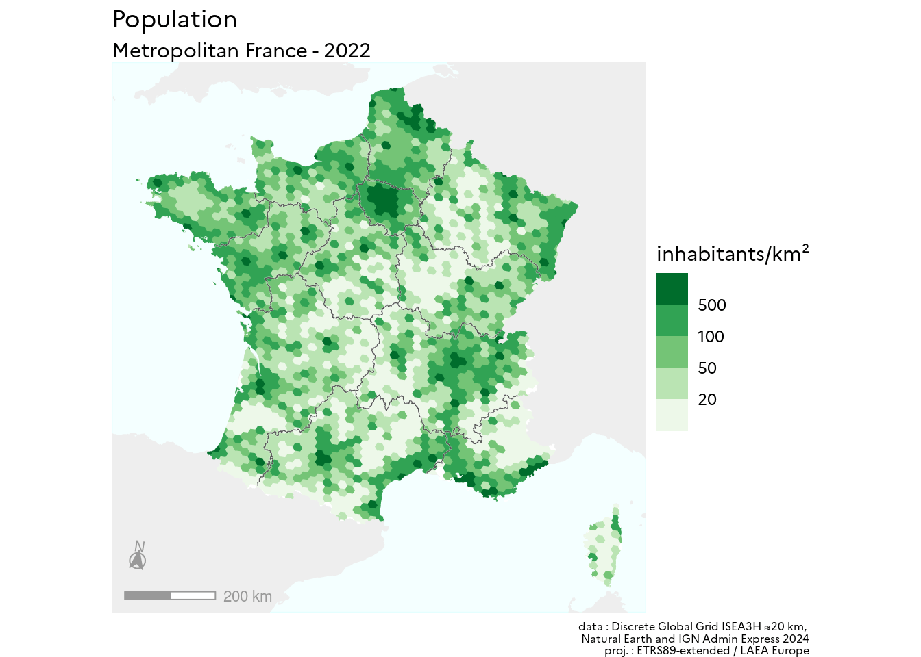
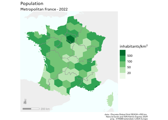
Now we can demonstrate our different resolutions:
build_map(20)


build_map(100)


