Generating a triangular navigation mesh from H3 hexagons in R

Introduction

A navigation mesh is a
data structure used to aid in pathfinding around obstacles. Originally
used for video games and robotics, we can also apply the concept of this
navigational mesh to the movement of animals through landscape, using
methods such as FEEMS.

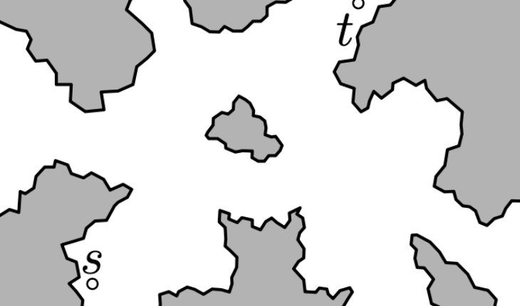
Consider the following landscape:

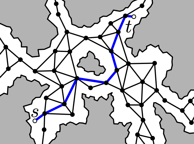
Finding a path from starting point s to goal point t is
computationally challenging, as there are many possible routes one might
take between these two endpoints, and the possibility space is so large
that it can be challenging to efficiently compute a fast path. Instead,
we can simplify the space by shrinking the possible locations in the
landscape to a series of nodes, and the neighboring nodes that you can
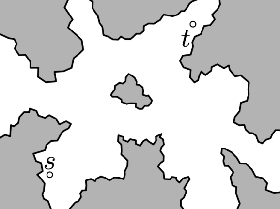
move to are connected by edges. The resulting mesh typically looks
like a bunch of triangles overlapping the landscape:

In this blog post I’ll discuss how to construct such a mesh using
real-world shapefiles and the h3 library in R, which tessellates
hexagons across the globe at several resolutions. I also looked into
alternatives such as
dggridR but I found other
packages to not be satisfactory for a number of reasons (mostly speed).

To begin with, why h3, and why hexagons? The answer to this is that it
is very convenient to have a grid system that can be used for any place
on the planet, and having a variety of different resolutions makes it
convenient to analyze spatial data on scales ranging from
continent-level to city-level. Hexagons in particular have a nice
property where the distance from the center of one hexagon to its
neighboring hex is roughly equal.

Worked example

First, load some required packages, including h3jsr, which I found to
have a nicer interface than other h3 libraries for R.

library(tidyverse)
library(h3jsr)
library(sf)
requireNamespace("maps")

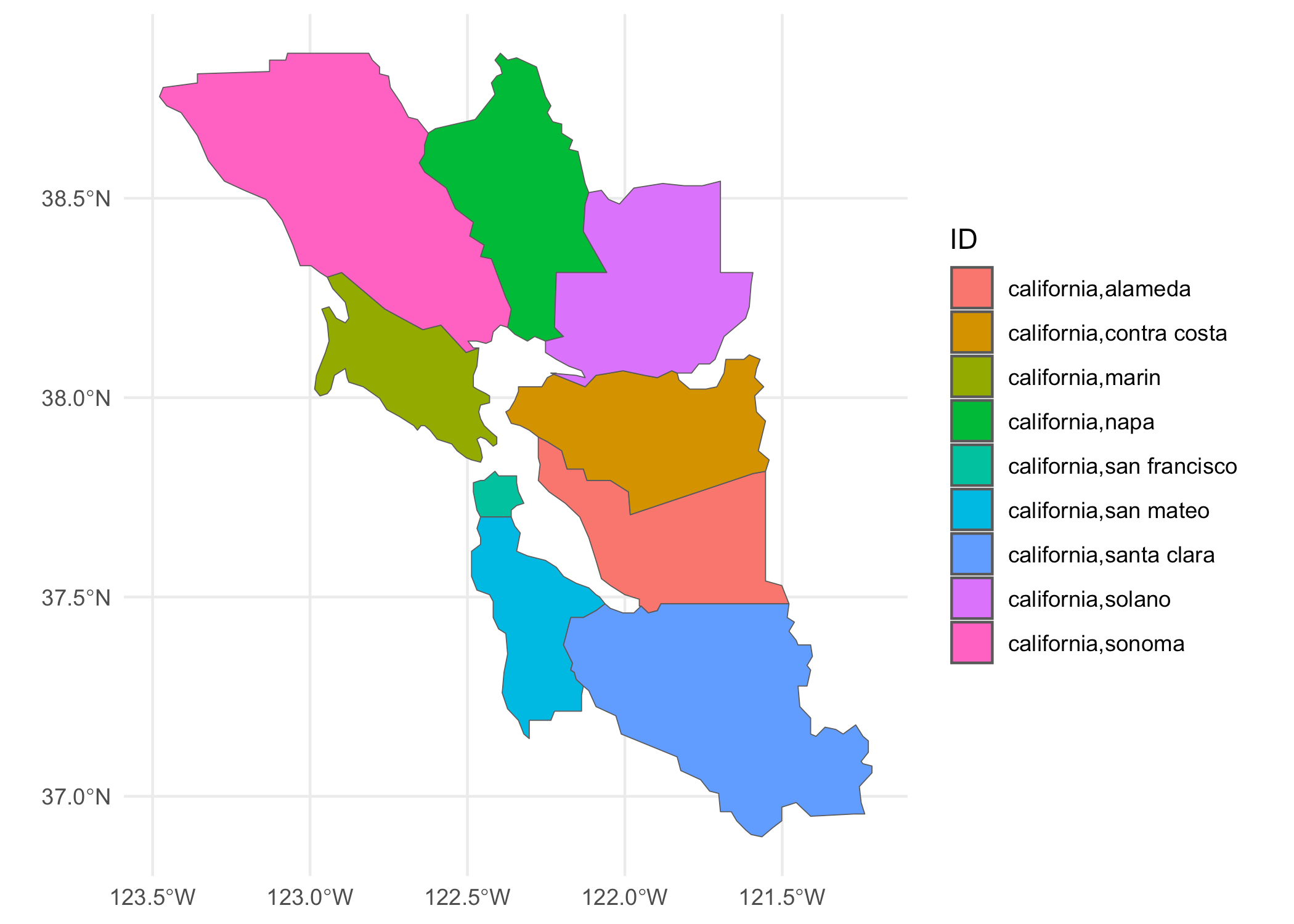
For today’s example we’ll be using a simple map showing some counties in
the San Francisco Bay Area (SFBA). We need to turn off spherical
geometry in sf since at this scale, everything is approximately planar
anyway and there are some issues with the geometries provided in the
maps package.

sf::sf_use_s2(FALSE)
bay_counties <- c(“alameda”, “contra costa”, “marin”, “napa”, “san mateo”, “santa clara”, “solano”, “sonoma”, “san francisco”)
sfba <- maps::map(‘county’, paste0(“california,”, bay_counties), fill = TRUE, plot = FALSE) %>%
st_as_sf() %>%
st_transform(4326) %>%
st_make_valid()
ggplot(sfba, aes(fill = ID)) +
geom_sf() +
theme_minimal()

Next, we need to find the h3 hexagons that intersect this shapefile of
the SFBA. I’d like my hexagons to cover a couple of square kilometers,
and this corresponds to roughly resolution
7 in
h3. We must first dissolve the individual features (i.e., remove
internal borders) then use the polygon_to_cells function to identify
the correct h3 cells that intersect with our SFBA borders.

dissolved_sfba <- summarise(sfba, geom = st_union(geom))
ids <- polygon_to_cells(dissolved_sfba, res = 7)[[1]]
head(ids)

## [1] "872830311ffffff" "872830925ffffff" "87283154dffffff" "872836a62ffffff"
## [5] "872830314ffffff" "872830928ffffff"

Plot these h3 hexes to get an idea of what we’re working with.

ggplot(cell_to_polygon(ids)) +
  geom_sf() +
  theme_minimal()

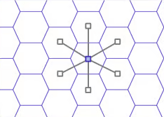
For each cell ID, we need to identify its neighbors using the get_disk
function with distance = 1. This function’s
documentation
says:

The first address returned is the input address, the rest follow in a
spiral anticlockwise order.

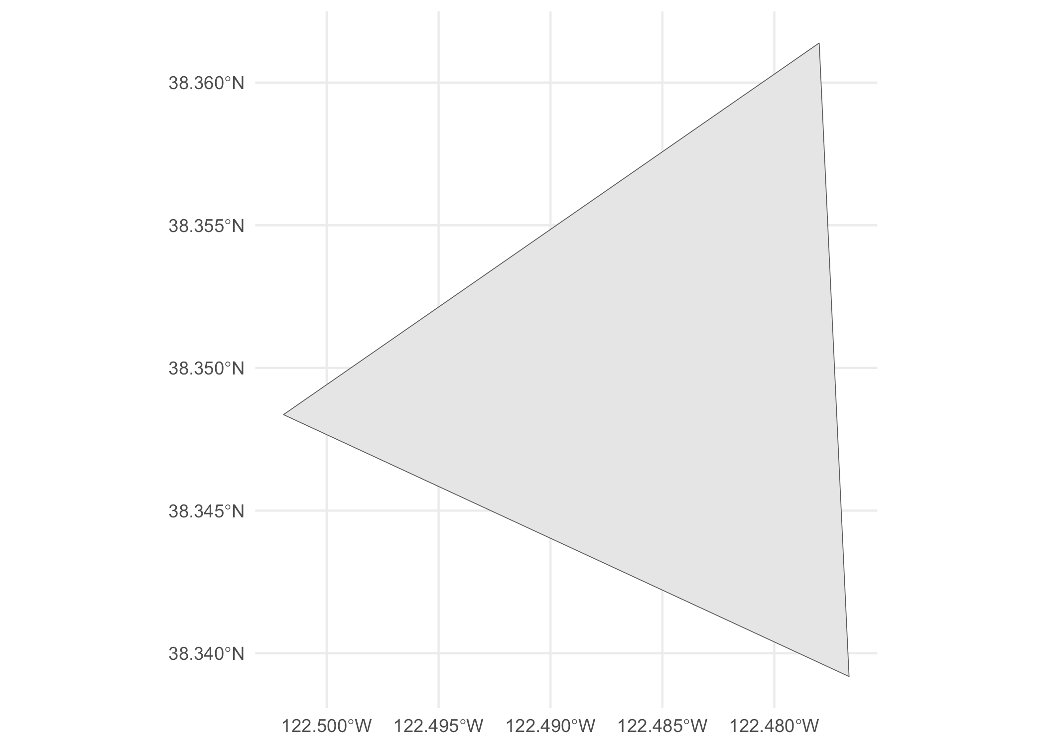
This is perfect for our use case. We take the origin hex and find its
center. Then do the same for two of its neighbors, and construct a
triangle between the centers of these three hexes.

id <- ids[1]
disk <- get_disk(id, ring_size = 1)[[1]]
first_three <- disk[1:3]
first_triangle <- cell_to_point(first_three, simple = TRUE) %>%
st_combine() %>%
st_cast(“POLYGON”) %>%
st_as_sf()
ggplot(first_triangle) +
geom_sf() +
theme_minimal()

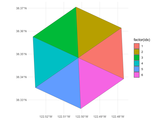
We can repeat this procedure to construct triangles between the centers
of all the hexes surrounding our origin hex. We exclude the origin point
from the loop and also add in the first neighboring hex in the ring,
otherwise we’ll only have five triangles, not six, around the origin
hex.

wrapped_vec <- c(disk[-1], disk[2])
results <- list()
for (ii in 1:(length(wrapped_vec) - 1)) {
results[[ii]] <- cell_to_point(c(id, wrapped_vec[ii], wrapped_vec[ii+1]), simple = TRUE) %>%
st_combine() %>%
st_cast(“POLYGON”) %>%
st_as_sf()
}
tris <- bind_rows(results) %>%
mutate(idx = 1:6)
ggplot(tris, aes(fill = factor(idx))) +
geom_sf() +
theme_minimal()

We can build off of this initial work to write a function that will take
an h3 id as input and return a triangular mesh.

to_triangles <- function(id) {
  disk <- get_disk(id, ring_size = 1)[[1]]
  wrapped_vec <- c(disk[-1], disk[2])
  lapply(1:(length(wrapped_vec) - 1), function(ii) {
    tri <- c(id, wrapped_vec[ii], wrapped_vec[ii + 1])
    cell_to_point(tri, simple = TRUE) %>%
      st_combine() %>%
      st_cast("POLYGON") %>%
      st_as_sf()
  }) %>% bind_rows()
}

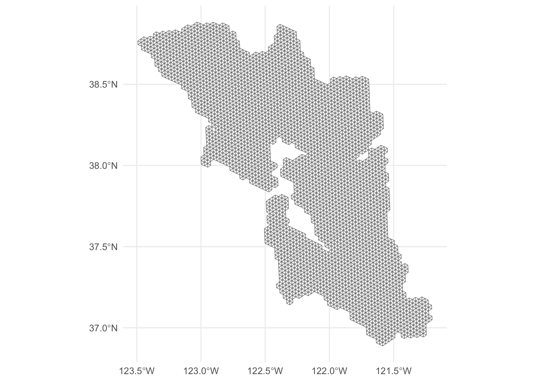
Use lapply and bind_rows to construct an entire sf dataframe that
contains the entire triangular mesh. There are a lot of duplicates but
we can just use distinct to get rid of these. (I use
parallel::mclapply here as this step can be a bit slow.)

all_tris <- parallel::mclapply(ids, to_triangles, mc.cores = 8) %>%
  bind_rows() %>%
  distinct()
ggplot(all_tris) +
geom_sf(fill = “white”) +
theme_minimal()

Observant readers will note that these triangle meshes will include
nodes that are out in the water or in neighboring counties, since the
hexes at the edge of our SFBA shapefile will inevitably have a few
neighbors that are not contained within the SFBA shapefile.

While it wasn’t necessary to do so for my analysis, these can easily be
removed by using a binary predicate such as st_contains, to never
include any edge that enters the water or otherwise exits the boundary
of the shapefile.

contain_result <- st_contains(dissolved_sfba, all_tris)
contained_mesh <- all_tris[unlist(contain_result), ]
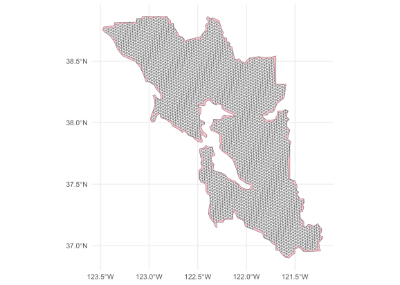
ggplot() +
  geom_sf(data = dissolved_sfba, fill = "pink") +
  geom_sf(data = contained_mesh, fill = "white") +
  theme_minimal()

This navigational mesh can now be saved using functions such as
write_sf and used in downstream analysis software.

Exercises

1. How can we avoid the creation of duplicate triangle meshes?
2. Use a compact representation to generate a triangle mesh with
   simplified interiors.

comp <- cell_to_polygon(h3jsr::compact(ids), simple = FALSE)
ggplot() +
geom_sf(data = dissolved_sfba, fill = NA) +
geom_sf(data = comp, fill = NA, color = “red”) +
theme_minimal()

Related