This is the fifth part of a blog post series on comparing spatial patterns in raster data. More information about the whole series can be found in part one.
This blog post focuses on comparing spatial patterns in categorical raster data for arbitrary regions. This means that the methods shown can be applied to compare rasters of the same region (for example, with the same resolution) and rasters of different regions (extents), resolutions, etc. This implies that the outcome of such comparisons is a single value, which indicates the difference/similarity between the spatial patterns of the two rasters.
Comparisons of arbitrary regions allow us to perform various types of spatial pattern analysis, including the search for similar regions or the grouping of regions based on their spatial patterns.
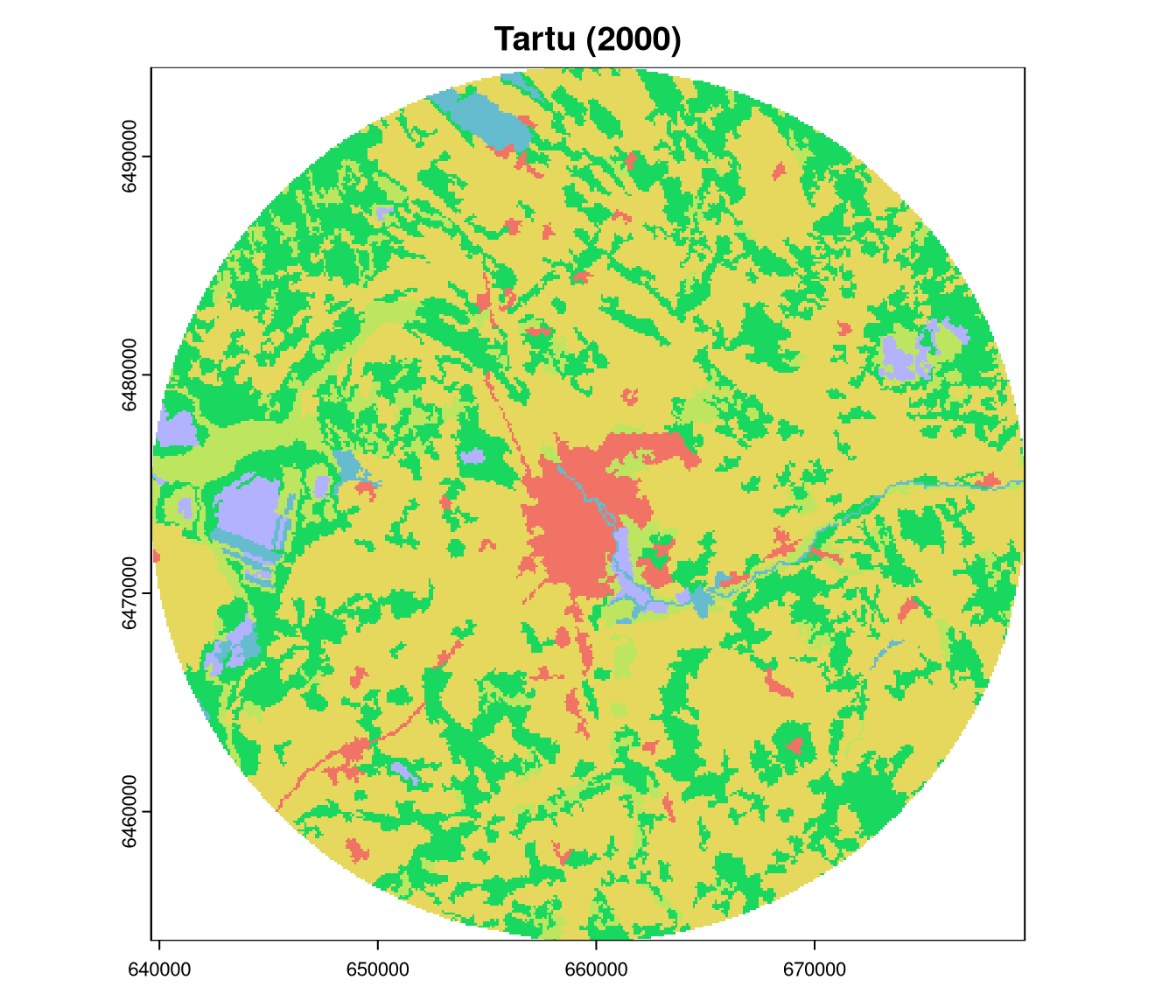
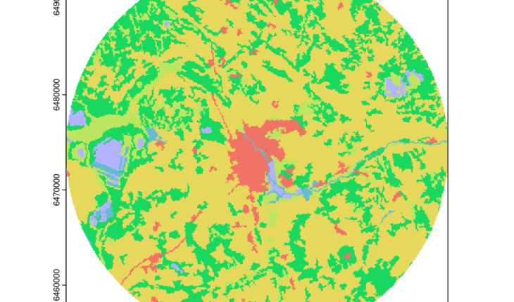
For this blog post, we use three categorical raster datasets: the CORINE Land Cover (CLC) datasets for Tartu (Estonia) for the years 2000 and 2018 and Poznań (Poland) for the year 2018.
library(terra)
clc2000_tartu = rast("https://github.com/Nowosad/comparing-spatial-patterns-2024/raw/refs/heads/main/data/clc2000_tartu.tif")
clc2018_tartu = rast("https://github.com/Nowosad/comparing-spatial-patterns-2024/raw/refs/heads/main/data/clc2018_tartu.tif")
clc2018_poznan = rast("https://github.com/Nowosad/comparing-spatial-patterns-2024/raw/refs/heads/main/data/clc2018_poznan.tif")
plot(clc2000_tartu, main = "Tartu (2000)")
plot(clc2018_tartu, main = "Tartu (2018)")
plot(clc2018_poznan, main = "Poznań (2018)")
The presented type of comparison can be done using information about the spatial context (e.g., the spatial arrangement of the categories; non-spatial context) or without it (e.g., non-spatial context). We start with the latter.
Non-spatial context
Single value outcome
Comparison of the values of a non-spatial landscape metric
Landscape metrics are a common way to quantify the spatial pattern of categorical raster data. Hundreds of such metrics exist, with each indicating a different aspect of the pattern of the landscape.1 Importantly, some metrics are sensitive to the spatial arrangement of the categories, while others are not. An example of a non-spatial metric is Shannon’s diversity index (SHDI), which quantifies the diversity of the landscape based on the number of categories and their proportions. The larger the value of SHDI, the more diverse the landscape is.
Now, if we calculate the SHDI for the two rasters, we can compare the values to see how different the diversity of the landscapes is. The new value indicates the difference in the diversity of the two landscapes.
library(landscapemetrics)
clc2000_tartu_shdi = lsm_l_shdi(clc2000_tartu)    # 1.15
clc2018_tartu_shdi = lsm_l_shdi(clc2018_tartu)    # 1.19
clc2018_poznan_shdi = lsm_l_shdi(clc2018_poznan)  # 1.21
abs(clc2018_tartu_shdi$value - clc2000_tartu_shdi$value)
abs(clc2018_poznan_shdi$value - clc2000_tartu_shdi$value)
abs(clc2018_poznan_shdi$value - clc2018_tartu_shdi$value)
Here, the results show that: a) the diversity of the Tartu landscape has increased between 2000 and 2018, b) the diversity of the Poznań landscape is larger than the Tartu landscape in 2018, and c) at the same time, the most similar landscapes are Tartu in 2018 and Poznań in 2018.
Spatial context
Single value outcome
Comparison of the values of a landscape metric
Many existing landscape metrics can also be used to quantify the pattern of categorical raster data with the spatial context. For example, the edge density (ED) metric quantifies the amount of edge in the landscape (where, edge is a length of the border between two categories). The larger the value of ED, the more edges the landscape has – this can be interpreted as a more fragmented landscape.
The difference between ED for the two rasters indicates how differently fragmented the landscapes are.
library(landscapemetrics)
clc2000_tartu_ed = lsm_l_ed(clc2000_tartu)    # 24.7
clc2018_tartu_ed = lsm_l_ed(clc2018_tartu)    # 24.6
clc2018_poznan_ed = lsm_l_ed(clc2018_poznan)  # 18.9
abs(clc2018_tartu_ed$value - clc2000_tartu_ed$value)
abs(clc2018_poznan_ed$value - clc2000_tartu_ed$value)
abs(clc2018_poznan_ed$value - clc2018_tartu_ed$value)
These comparisons show a different perspective on the landscapes: a) the fragmentation of the Tartu landscape (almost) has not changed between 2000 and 2018, b) the Poznań landscape is less fragmented than the Tartu landscape in 2018, and c) the most different landscapes are Tartu in 2018 and Poznań in 2018.
The above examples use the landscapemetrics package (Hesselbarth et al. 2019).
Comparison of the values of Zhao’s entropy for landscape mosaics
Recently, several new metrics related to the complexity of the landscapes have been proposed.2 For categorical rasters, it includes Zhao’s entropy metric (Zhao and Zhang 2019). The larger the value of Zhao’s entropy, the more complex the landscape is. Thus, the absolute difference between the values of Zhao’s entropy for two rasters indicates how differently complex the landscapes are, with low values indicating similar complexity and high values indicating different complexity.
library(bespatial)
clc2000_tartu_bes = bes_m_zhao(clc2000_tartu)   # 0.0372
clc2018_tartu_bes = bes_m_zhao(clc2018_tartu)   # 0.0385
clc2018_poznan_bes = bes_m_zhao(clc2018_poznan) # 0.0406
abs(clc2018_tartu_bes$value - clc2000_tartu_bes$value)
abs(clc2018_poznan_bes$value - clc2000_tartu_bes$value)
abs(clc2018_poznan_bes$value - clc2018_tartu_bes$value)
This complexity measure suggests that both rasters for Tartu have similar complexity, while the Poznań raster is more complex than the Tartu rasters. Moreover, the most different landscapes are Tartu in 2000 and Poznań in 2018.
This example uses the bespatial package (Nowosad 2024).
Dissimilarity of a spatial signature between two rasters
An alternative approach to the use of a single landscape metric for comparing spatial patterns in categorical raster data of arbitrary regions is to calculate a spatial signature of the landscape. A spatial signature is a vector of values that describe the spatial pattern of the landscape. Such a signature may be based on a co-occurrence vector (cove; a vector that shows how often each pair of categories is adjacent to each other). Next, the spatial signatures for two rasters can be compared using a distance measure, such as the Jensen-Shannon divergence (Jasiewicz and Stepinski 2013). The smaller the outcome value, the more similar the spatial patterns of the two rasters are.
The spatial signature can be calculated using the motif package (Nowosad 2021) and compared with the philentropy package (HG 2018).
library(motif)
library(philentropy)
clc2000_tartu_sign = lsp_signature(clc2000_tartu, type = "cove", threshold = 1)
clc2018_tartu_sign = lsp_signature(clc2018_tartu, type = "cove", threshold = 1)
clc2018_poznan_sign = lsp_signature(clc2018_poznan, type = "cove", threshold = 1)
jensen_shannon(clc2000_tartu_sign$signature[[1]],
               clc2018_tartu_sign$signature[[1]],
               testNA = FALSE, unit = "log2")       # 0.0011
jensen_shannon(clc2000_tartu_sign$signature[[1]],
               clc2018_poznan_sign$signature[[1]],
               testNA = FALSE, unit = "log2")       # 0.0912
jensen_shannon(clc2018_tartu_sign$signature[[1]],
               clc2018_poznan_sign$signature[[1]],
               testNA = FALSE, unit = "log2")       # 0.0826
Here, using this spatial signature, we can see that the Tartu landscapes are much more similar to each other than to the Poznań landscape.
References
HG, Drost. 2018. “Philentropy: Information Theory and Distance Quantification with R.” Journal of Open Source Software 3 (26): 765.
———. 2024. Bespatial: Boltzmann Entropy for Spatial Data. Manual.
Reuse
Citation
BibTeX citation:
@online{nowosad2024,
  author = {Nowosad, Jakub},
  title = {Comparison of Spatial Patterns in Categorical Raster Data for
    Arbitrary Regions Using {R}},
  date = {2024-11-10},
  url = {https://jakubnowosad.com/posts/2024-11-10-spatcomp-bp5/},
  langid = {en}
}
For attribution, please cite this work as:
Categorical Raster Data for Arbitrary Regions Using R.” November
10, 2024. https://jakubnowosad.com/posts/2024-11-10-spatcomp-bp5/.
Related


