A Bayesian proportional hazards model with a penalized spline

Simulating data with a time-varying hazard ratio

Here are the R packages used in the post:

library(simstudy)
library(ggplot2)
library(data.table)
library(survival)
library(survminer)
library(splines)
library(splines2)
library(cmdstanr)

The dataset simulates a randomized controlled trial in which patients are assigned either to the treatment group (\(A=1\)) or control group (\(A=0\)) in a \(1:1\) ratio. Patients enroll over nine quarters, with the enrollment quarter denoted by \(M\), \(M \in \{0, \dots, 8 \}\). The time-to-event outcome, \(Y\), depends on both treatment assignment and enrollment quarter. To introduce non-linearity, I define the relationship using a cubic function, with true parameters specified as follows:

defI <- 
  defData(varname = "A", formula = "1;1", dist = "trtAssign") |>
  defData(varname = "M", formula = "0;8", dist = "uniformInt")

defS <-
  defSurv(
    varname = "eventTime",
    formula = "..int + ..beta * A + ..alpha_1 * M + ..alpha_2 * M^2 + ..alpha_3 * M^3",
    shape = 0.30)  |>
  defSurv(varname = "censorTime", formula = -11.3, shape = 0.40)

# parameters

int <- -11.6      
beta <-  0.70
alpha_1 <-  0.10   
alpha_2 <-  0.40    
alpha_3 <- -0.05

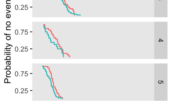
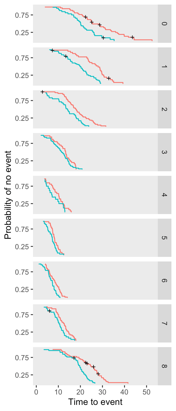
I’ve generated a single data set of \(640\) study participants, \(320\) in each arm. The plot below shows the Kaplan-Meier curves by arm for each enrollment period.

set.seed(7368) # 7362

dd <- genData(640, defI)
dd <- genSurv(dd, defS, timeName = "Y", censorName = "censorTime",
  eventName = "event", typeName = "eventType", keepEvents = TRUE)

Bayesian model

This Bayesian proportional hazards model builds directly on the approach from my previous post. Since the effect of \(M\) on \(Y\) follows a non-linear pattern, I model this relationship using a spline to account for temporal variation in the hazard. The partial likelihood is a function of the treatment effect and spline basis function coefficients, given by:

\[
L(\beta,\mathbf{\gamma}) = \prod_{i=1}^{N} \left( \frac{\exp \left(\beta A_i + \sum_{m=1} ^ M \gamma_m X_{m_i} \right)} {\sum_{j \in R(t_i)} \exp\left(\beta A_j + \sum_{m=1} ^ M \gamma_m X_{m_j}\right) } \right)^{\delta_i}
\]
where:

• \(M\): number of spline basis functions
• \(N\): number of observations (censored or not)
• \(A_i\): binary indicator for treatment
• \(X_{m_i}\): value of the \(m^{\text{th}}\) spline basis function for the \(i^{\text{th}}\) observation
• \(\delta_i\): event indicator (\(\delta_i = 1\) if the event occurred, \(\delta_i = 0\) if censored)
• \(\beta\): treatment coefficient
• \(\gamma_m\): spline coefficient for the \(m^\text{th}\) spline basis function
• \(R(t_i)\): risk set at time \(t_i\) (including only individuals censored after \(t_i\))

The spline component of the model is adapted from a model I described last year. In this formulation, time-to-event is modeled as a function of the vector \(\mathbf{X_i}\) rather than the period itself. The number of basis functions is determined by the number of knots, with each segment of the curve estimated using B-spline basis functions. To minimize overfitting, we include a penalization term based on the second derivative of the B-spline basis functions. The strength of this penalization is controlled by a tuning parameter, \(\lambda\), which is provided to the model.

The Stan code, provided in full here, was explained in earlier posts. The principal difference from the previous post is the addition of the spline-related data and parameters, as well as the penalization term in the model.:

stan_code <-
"
functions {

  // Binary search optimized to return the last index with the target value

  int binary_search(vector v, real tar_val) {
    int low = 1;
    int high = num_elements(v);
    int result = -1;

    while (low <= high) {
      int mid = (low + high) %/% 2;
      if (v[mid] == tar_val) {
        result = mid; // Store the index
        high = mid - 1; // Look for earlier occurrences
      } else if (v[mid] < tar_val) {
        low = mid + 1;
      } else {
        high = mid - 1;
      }
    }
    return result;
  }
}

data {

  int K;          // Number of covariates
  int N_o;        // Number of uncensored observations
  vector[N_o] t_o;         // Event times (sorted in decreasing order)

  int N;          // Number of total observations
  vector[N] t;             // Individual times (sorted in decreasing order)
  matrix[N, K] x;          // Covariates for all observations

  // Spline-related data
  
  int Q;          // Number of basis functions
  matrix[N, Q] B;          // Spline basis matrix
  matrix[N, Q] D2_spline;  // 2nd derivative for penalization
  real lambda;             // penalization term
}

parameters {
  vector[K] beta;          // Fixed effects for covariates
  vector[Q] gamma;         // Spline coefficients
}

model {
  
  // Prior
  
  beta ~ normal(0, 4);
  
  // Spline coefficients prior
  
  gamma ~ normal(0, 4);
  
  // Penalization term for spline second derivative
  
  target += -lambda * sum(square(D2_spline * gamma));
  
  // Calculate theta for each observation to be used in likelihood
  
  vector[N] theta;
  vector[N] log_sum_exp_theta;
  
  for (i in 1:N) {
    theta[i] = dot_product(x[i], beta) + dot_product(B[i], gamma);  
  }
  
  // Compute cumulative sum of log(exp(theta)) from last to first observation
  
  log_sum_exp_theta[N] = theta[N];
  
  for (i in tail(sort_indices_desc(t), N-1)) {
    log_sum_exp_theta[i] = log_sum_exp(theta[i], log_sum_exp_theta[i + 1]);
  }

  // Likelihood for uncensored observations
  
  for (n_o in 1:N_o) {
    int start_risk = binary_search(t, t_o[n_o]); // Use binary search
    
    real log_denom = log_sum_exp_theta[start_risk];
    target += theta[start_risk] - log_denom;
  }
}
"

To estimate the model, we need to get the data ready to pass to Stan, compile the Stan code, and then sample from the model using cmdstanr:

dx <- copy(dd)
setorder(dx, Y)

dx.obs <- dx[event == 1]
N_obs <- dx.obs[, .N]
t_obs <- dx.obs[, Y]

N_all <- dx[, .N]
t_all <- dx[, Y]
x_all <- data.frame(dx[, .(A)])

# Spline-related info

n_knots <- 5
spline_degree <- 3
knot_dist <- 1/(n_knots + 1)
probs <- seq(knot_dist, 1 - knot_dist, by = knot_dist)
knots <- quantile(dx$M, probs = probs)
spline_basis <- bs(dx$M, knots = knots, degree = spline_degree, intercept = TRUE)
B <- as.matrix(spline_basis)

D2 <- dbs(dx$M, knots = knots, degree = spline_degree, derivs = 2, intercept = TRUE)
D2_spline <- as.matrix(D2)

K <- ncol(x_all)             # num covariates - in this case just A

stan_data <- list(
  K = K,
  N_o = N_obs,
  t_o = t_obs,
  N = N_all,
  t = t_all,
  x = x_all,
  Q = ncol(B),
  B = B,
  D2_spline = D2_spline,
  lambda = 0.10
)

# compiling code

stan_model <- cmdstan_model(write_stan_file(stan_code))

# sampling from model

fit <- stan_model$sample(
  data = stan_data,
  iter_warmup = 1000,
  iter_sampling = 4000,
  chains = 4,
  parallel_chains = 4,
  max_treedepth = 15,
  refresh = 0
)
## Running MCMC with 4 parallel chains...
## 
## Chain 4 finished in 64.1 seconds.
## Chain 3 finished in 64.5 seconds.
## Chain 2 finished in 65.2 seconds.
## Chain 1 finished in 70.6 seconds.
## 
## All 4 chains finished successfully.
## Mean chain execution time: 66.1 seconds.
## Total execution time: 70.8 seconds.

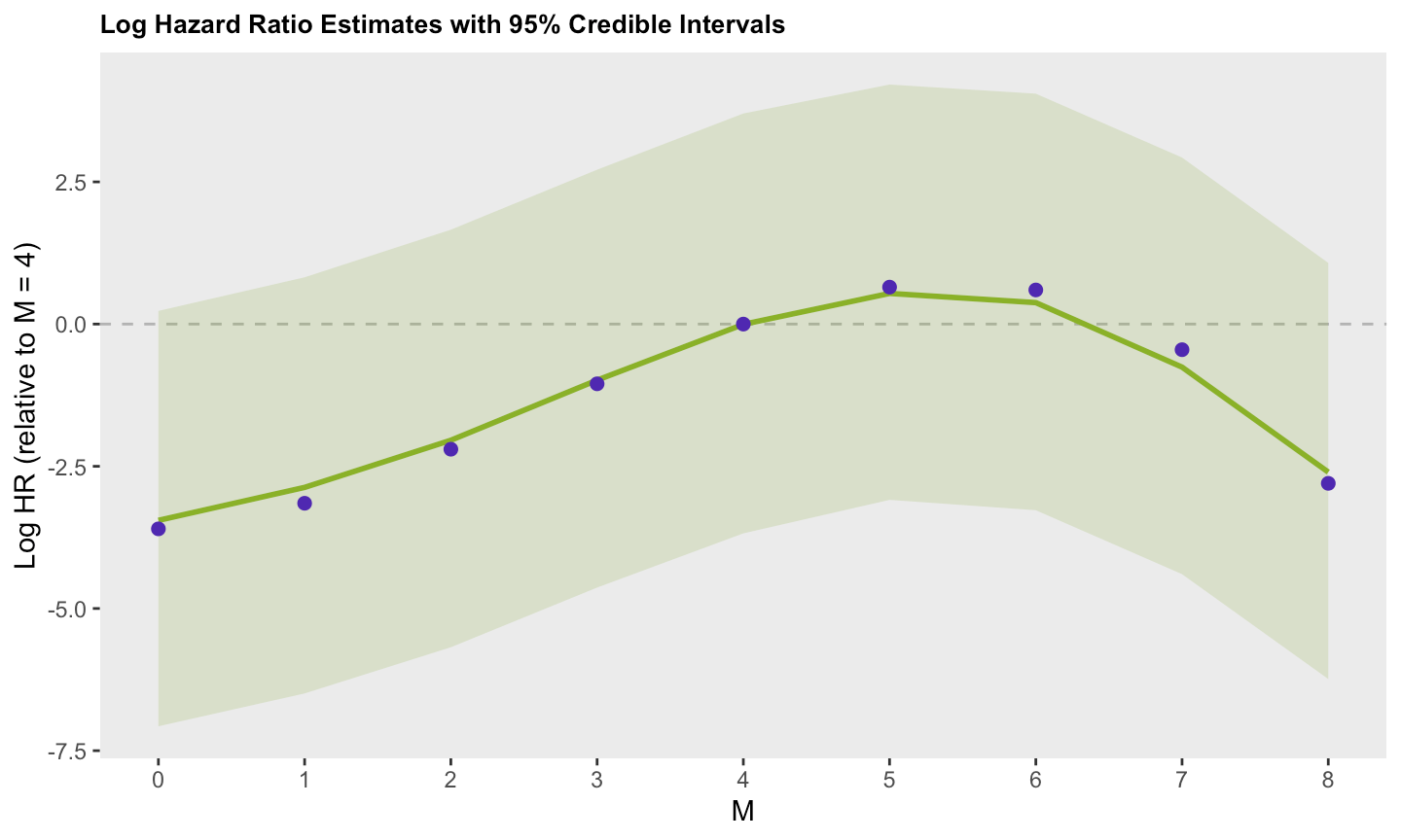
The posterior mean (and median) for \(\beta\), the treatment effect, are quite close to the “true” value of 0.70:

fit$summary(variables = c("beta", "gamma"))
## # A tibble: 10 × 10
##    variable   mean median     sd    mad     q5   q95  rhat ess_bulk ess_tail
##                           
##  1 beta[1]   0.689  0.689 0.0844 0.0857  0.551 0.828  1.00    3664.    4002.
##  2 gamma[1] -1.75  -1.77  1.33   1.35   -3.91  0.468  1.00    1364.    1586.
##  3 gamma[2] -1.59  -1.60  1.33   1.35   -3.75  0.626  1.00    1360.    1551.
##  4 gamma[3] -1.22  -1.24  1.33   1.35   -3.39  0.978  1.00    1365.    1515.
##  5 gamma[4] -0.115 -0.127 1.33   1.35   -2.28  2.09   1.00    1361.    1576.
##  6 gamma[5]  1.97   1.95  1.34   1.35   -0.206 4.20   1.00    1366.    1581.
##  7 gamma[6]  2.63   2.61  1.33   1.34    0.452 4.84   1.00    1358.    1586.
##  8 gamma[7]  1.08   1.05  1.33   1.34   -1.08  3.28   1.00    1360.    1505.
##  9 gamma[8] -0.238 -0.260 1.33   1.34   -2.40  1.97   1.00    1355.    1543.
## 10 gamma[9] -0.914 -0.935 1.33   1.35   -3.07  1.30   1.00    1356.    1549.

The figure below shows the estimated spline and the 95% credible interval. The green line represents the posterior median log hazard ratio for each period (relative to the middle period, 4), with the shaded band indicating the corresponding credible interval. The purple points represent the log hazard ratios implied by the data generation process. For example, the log hazard ratio comparing period 1 to period 4 for both arms is:

\[
\begin{array}{c}
(-11.6 + 0.70A +0.10\times1 + 0.40 \times 1^2 -0.05\times1^3) – (-11.6 + 0.70A +0.10\times4 + 0.40 \times 4^2 -0.05\times4^3) = \\
(0.10 + 0.40 – 0.05) – (0.10 \times 4 + 0.40 \times 16 – 0.05 \times 64 ) = \\
0.45 – 3.60 = -3.15
\end{array}
\]

It appears that the median posterior aligns quite well with the values used in the data generation process:

For the next post, I will present another scenario that includes random effects for a cluster randomized trial (but will not include splines).