Smith-Pittman Algorithm: Enhancing Community Detection in Networks

Introduction

Social network analysis examines individual entities and their relationships among them. The data is represented as a “graph” where individual entities are referred to as “nodes” and their relationships between them as “edges. A primary area of study in SNA is the analysis of interconnectivity of nodes, called ”communities” and identification of clusters through the use of algorithms called ”community detection algorithms”.

I was lucky enough to develop an community detection algorithm with Tyler Pittman under the supervision of Dr. Wei Xu and which proved to offer “more descriptive” community identification in certain settings when compared to other algorithms – such as the Girvan-Newman and Louvain algorithms. To make the algorithm readily available for other users, the {ig.degree.betweenness} R package was created. If you want to learn about the setting for which the algorithm was originally developed, check out the arXiv preprint here.

The {ig.degree.betweenness} package provides an implementation of the “Smith-Pittman” community detection algorithm for igraph users in R. It can be installed directly from CRAN by running:

install.packages("ig.degree.betweenness")

Alternatively, it can be installed from the GitHub repository with the {devtools} package:

# Install the devtools package if you haven't installed it
# install.packages("devtools")
devtools::install_github("benyamindsmith/ig.degree.betweenness")

The Smith-Pittman Algorithm

The algorithm can be thought of as an extension of the Girvan-Newman algorithm that also considers both degree centrality – a.k.a the number of connections possessed by each individual node in the network and edge-betweenness – a.k.a. the number of shortest paths that pass through each individual edge in the network.

The steps for the algorithm are:

1. Identify the node with the highest degree-centrality in the network (the “most popular” node)
2. Select the subgraph of the node with the highest degree centrality. Remove the edge possessing the highest calculated (network-wide) edge-betweenness in the subgraph.
3. Recalculate the degree centrality for all nodes in the network and the betweenness for the remaining edge in the network.
4. Repeat from step 2.

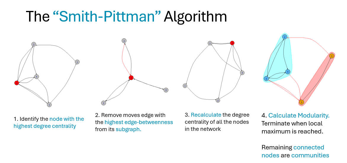
Conceptually, this algorithm (similar to Girvan-Newman and Louvain) can be specified to terminate once a pre-determined number of communities has been identified (based on the remaining connected nodes). However, the intention for using this algorithm is meant to be used in an unsupervised, modularity maximizing setting, where the grouping of nodes is decided on the strength of the connected clusters.

Applications of the Smith-Pittman algorithm

The Smith-Pittman algorithm thrives in certain settings where other methods fail. In particular the Smith Pittman algorithm appears to do well in identifying communities of descriptive value in settings where there is strong “popularity-hierarchy” present in terms of nodes in the network. The following are two examples where Smith-Pittman appears to fair better in terms of identifying descriptive communities than the Girvan-Newman and Louvain community detection algorithms.

Zachary’s Karate Club

The Zachary’s Karate Club dataset has become a classic dataset used for studying social network analysis and community detection. The split between members in the club is known and and serves as a good starting point for learning about and applying social network analysis. The data is readily available via the {igraphdata} package.

The initial network can be plotted with the following R code:

# Install relevant libraries for the entire analysis
library(igraph)
library(igraphdata)
library(ig.degree.betweenness)
# Setting seed for visual reproducibility
set.seed(5250)

par(mar=c(0,0,0,0)+2)
data("karate")

plot(karate, main ="Zachary's Karate Club")

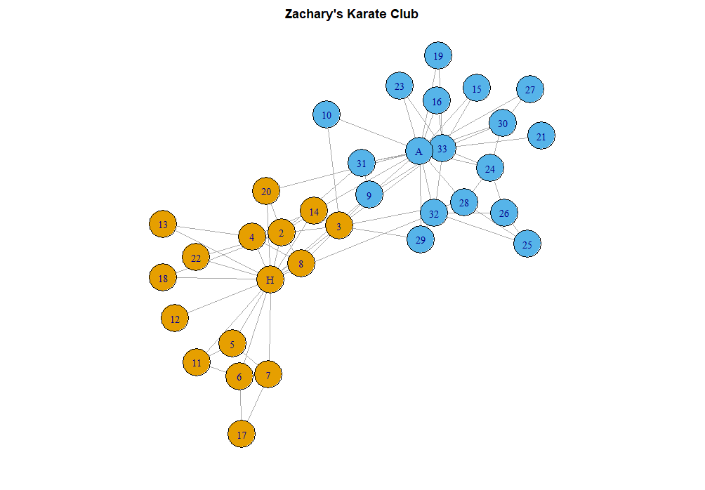
In the context of community detection, the object of interest is seeing if the split of members in the club could be identified based on the relationships between members in the network. For comparing the community detection algorithms, the following code is used:

# Girvan-Newman communities
gn_karate <- karate |>
  igraph::cluster_edge_betweenness()
# Louvain communities
louvain_karate <- karate |>
  igraph::cluster_louvain()
# Smith-Pittman Communities
sp_karate <- karate |>
  ig.degree.betweenness::cluster_degree_betweenness()

#Plotting all 3 visuals
par(mfrow= c(1,3),mar=c(0,0,0,0)+2)
set.seed(5250)
plot(gn_karate,
  karate,
  main = "Girvan-Newman"
  )
set.seed(5250)
plot(
  louvain_karate,
  karate,
  main = "Louvain"
)
set.seed(5250)
plot(
  sp_karate,
  karate,
  main = "Smith-Pittman"
)

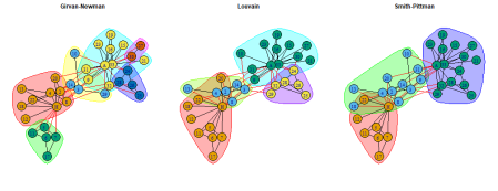
When applied in an unsupervised setting, the Girvan-Newman and Louvain algorithms identify communities of nodes which optimize modularity according to their approaches. However, the communities identified do not appear to identify a possible division in the group which is contextually informative or interpretative. The Smith-Pittman algorithm identifies 3 communities which could can be understood as individuals who would certainly associate with John A. or Mr. Hi and an uncertain group.

To justify the rationale for Smith-Pittman further, the network with the communities identified and the nodes resized based on the number of connections possessed (degree centrality) can be viewed with the following code:

set.seed(5250)
VS <- igraph::degree(karate)
plot(
    sp_karate,
     karate,
     vertex.size=VS,
     main = "Smith-Pittman Communities with Node Resizing"
)

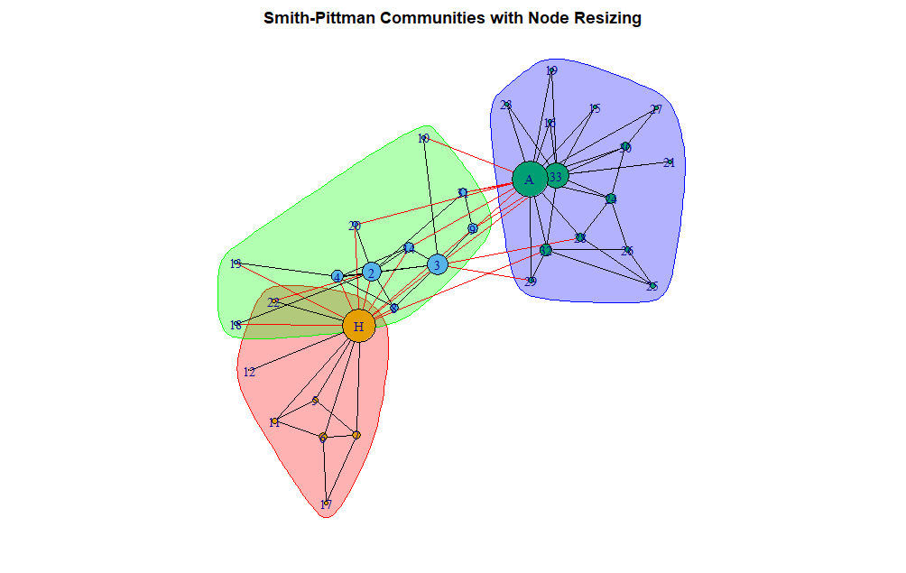
This visual offers some evidence to the rationale for how the algorithm partitioned the individuals in the club.

TidyTuesday – “Monster Movies” dataset

The “Monster Movies” dataset, made available by the TidyTuesday project presents an interesting example for applying SNA and the Smith-Pitman algorithm to the interaction between genres in “monster” titled movies. To plot a “simplified” network with node sizes corresponding to the number of connections, the following code is used:

# Install relevant libraries
# pkgs <- c("dplyr","tibble","tidyr","tidygraph", 
#           "igraph","ig.degree.betweenness")
# install.packages(pkgs)
# Load data
tuesdata <- tidytuesdayR::tt_load(2024, week = 44)
monster_movie_genres <- tuesdata$monster_movie_genres

# Prepare data for adjacency matrix
dummy_matrix <- monster_movie_genres |>
  dplyr::mutate(value = 1) |>
  tidyr::pivot_wider(
    id_cols = tconst,
    names_from = genres,
    values_from = value,
    values_fill = 0
  ) |>
  dplyr::select(-tconst) |>
  as.matrix.data.frame()

# Construct adjacency matrix
genre_adj_matrix <- t(dummy_matrix) %*% dummy_matrix
# Setting self loops to zero
diag(genre_adj_matrix) <- 0

# Construct the graph
movie_graph <- genre_adj_matrix |>
  as.data.frame() |>
  tibble::rownames_to_column() |>
  tidyr::pivot_longer(cols = Comedy:War) |>
  dplyr::rename(c(from = rowname, to = name)) |>
  dplyr::rowwise() |>
  dplyr::mutate(combo = paste0(sort(c(from, to)), collapse = ",")) |>
  dplyr::arrange(combo) |>
  dplyr::distinct(combo, .keep_all = TRUE) |>
  dplyr::select(-combo) |>
  tidyr::uncount(value) |>
  tidygraph::as_tbl_graph()

# Resize nodes based on node degree

VS <- igraph::degree(movie_graph) * 0.1

ig.degree.betweenness::plot_simplified_edgeplot(
  movie_graph,
  vertex.size = VS,
  edge.arrow.size = 0.001
)

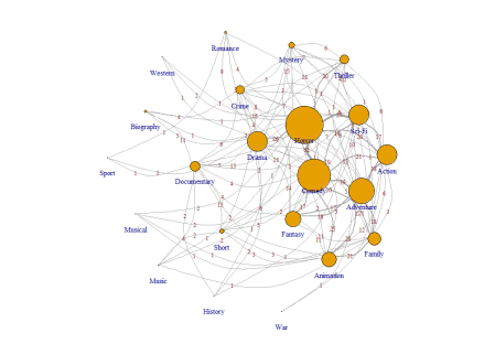
The edge thickness and annotated numbers correspond to the number of edges shared between listed genres. For plotting the genre clusters in the network as preformed by (a)-Girvan-Newman, (b)-Louvain and (c)-Smith-Pittman the following code is used:

# Cluster Nodes
gn_cluster <- movie_graph |>
  igraph::as.undirected() |>
  igraph::cluster_edge_betweenness()

louvain_cluster <- movie_graph |>
  igraph::as.undirected() |>
  igraph::cluster_louvain()

sp_cluster <- movie_graph |>
  igraph::as.undirected() |>
  ig.degree.betweenness::cluster_degree_betweenness()

# Figure 5
par(mfrow = c(1, 3), mar = c(0, 0, 0, 0) + 1)

ig.degree.betweenness::plot_simplified_edgeplot(
  movie_graph,
  gn_cluster,
  main = "(a)",
  vertex.size = VS,
  edge.arrow.size = 0.001
)

ig.degree.betweenness::plot_simplified_edgeplot(
  movie_graph,
  louvain_cluster,
  main = "(b)",
  vertex.size = VS,
  edge.arrow.size = 0.001
)

ig.degree.betweenness::plot_simplified_edgeplot(
    movie_graph,
    sp_cluster,
    main = "(c)",
    vertex.size = VS,
    edge.arrow.size = 0.001
)

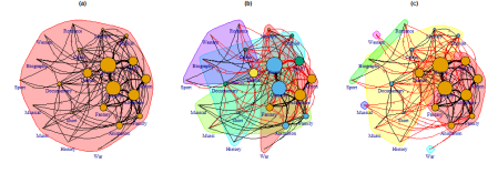
Girvan Newman fails to identify any communities in the network (clustering all genres in one group isn’t really community identification). Louvain might be telling us something in terms of strength of clustering but doesn’t necessarily speak about the reality of “monster” movie genre interactions. Smith-Pittman clustering tells the best story with popular genres forming the primary working group followed by more ambivalent smaller subgroups and outlier nodes.

Limitations

The Smith-Pittman algorithm preforms best in a setting where there are a high number of connections for the number of nodes in the network and a there is a diversity in degree centrality among the nodes. For a comically bad setting can be seen from a screenshot I had from a conversations on Discord:

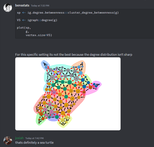
That being said, there is no specific model which describes exactly what a ”community” is. So where Smith-Pittman “fails”, another community detection algorithm might be more justified.

Conclusions

Thank you to my collaborators for helping develop this method, and thank you to everyone who has taken the time to check out the methodology. If you have used it or plan on using it, please let me know!

Related